Fan in a Duct (Actuator Disk with a Fan Curve)¶

Browse this case on GitHub

A step-by-step tutorial for the fan model of code_saturne: a virtual disk placed inside the mesh, pushing the flow according to a prescribed characteristic curve $\Delta P(Q)$: the everyday tool for ventilation studies where meshing the real fan is out of the question. A duct is closed into a periodic loop with a fan and a resistance screen: the flow rate is imposed nowhere, and the computation settles on the operating point, the intersection of the fan curve with the circuit load.

Maintained by Simvia, part of the tutoriel-code_saturne collection.

Learning objectives¶

After completing this tutorial you will be able to:

Define a fan from the GUI (Fans page): axis, radii, and the characteristic curve given by its three coefficients $\Delta P = C_0 + C_1 Q + C_2 Q^2$.
Know the two traps of the model: the pressure-jump mode (blades and hub radii at zero) versus the blade-profile mode, and the thrust conservation factor when the theoretical disk does not match the meshed section.
Read the operating point live in the log (Fans block) and verify it against the curve intersection.

Prerequisites¶

Requirement	Detail
code_saturne	v9.1
Tutorials	Inc_Head_Loss_Zone (the screen), Inc_Streamwise_Periodic (periodicity)

If code_saturne is not yet installed, build it from the official homepage, pull a ready-to-use Singularity image from the Open Simulation Center, or pull the Simvia Docker image before continuing.

Case files¶

Inc_Fan_Duct/
├── CASE/
│   └── DATA/setup.xml     # fan, screen, periodic loop: all GUI
├── FIGURES/               # figures used in this README
└── README.md

Built-in cartesian mesher, no user routine, no mesh file.

The case¶

A $1$ m duct of square section ($0.1 \times 0.1$ m, air, laminar) is closed into a periodic loop: no inlet, no outlet, so no boundary condition enters the balance. The loop carries two elements:

the fan ($x = 0.45$ to $0.55$ m), used in pressure-jump mode (blades and hub radii at zero: uniform axial push, the ideal actuator);
the screen, a head-loss zone: it stands for whatever a real fan must overcome (filter, coil, grilles, or a whole duct network aggregated into one coefficient) and gives the circuit its load curve $\Delta p = \frac{1}{2}\rho\,\zeta\,(Q/A)^2$. Its coefficient comes from the GUI head-loss zone exactly as in Inc_Head_Loss_Zone: $K_{xx} = 100\ \mathrm{m^{-1}}$ is a resistance per metre of zone, so the screen of thickness $L = 0.1$ m totals $\zeta = K_{xx} L = 10$: at the operating point, $\Delta p = \frac{1}{2} \times 1.2 \times 10 \times 1.768^2 = 18.75$ Pa.

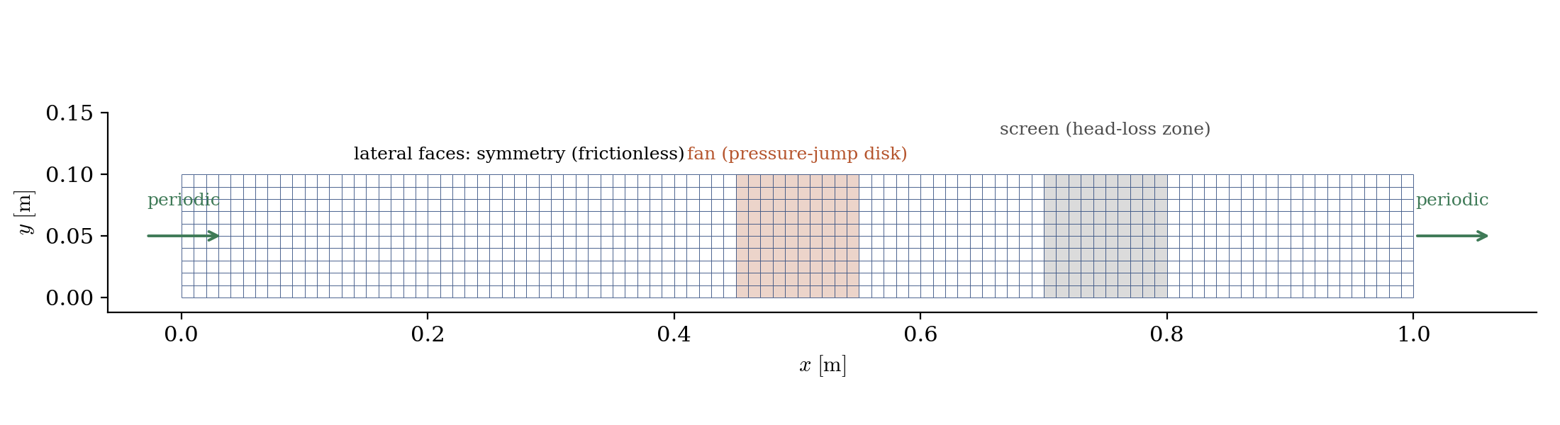
The periodic duct loop with its mesh, the fan disk and the head-loss screen highlighted.
Figure 1: the computational domain: a periodic duct loop with the fan disk (orange) and the resistance screen (grey); lateral faces are frictionless symmetries.

The fan curve $\Delta P = 50 - 10^5 Q^2$ is a didactic stand-in for a small axial fan: $50$ Pa at zero flow, free delivery at $22.4$ L/s. In a real study, the three coefficients are fitted on the manufacturer's curve. The negative slope is what makes the operating point stable.

How the curve enters the setup. The three coefficients are typed in the GUI Fans page and land in setup.xml as:

<curve_coeffs_x>24.868</curve_coeffs_x>     <!-- C0 [Pa] -->
<curve_coeffs_y>0.0</curve_coeffs_y>        <!-- C1 [Pa/(m3/s)] -->
<curve_coeffs_z>-49736.8</curve_coeffs_z>   <!-- C2 [Pa/(m3/s)2] -->

Beware the naming: the _x, _y, _z suffixes are not directions but the polynomial degrees $C_0$, $C_1$, $C_2$ of $\Delta P = C_0 + C_1 Q + C_2 Q^2$ ($Q$ in $\mathrm{m^3/s}$). At every iteration, the solver measures the flow $Q$ through the disk, evaluates $\Delta P(Q)$ from these coefficients, and applies the corresponding force: this feedback is what drives the run to the operating point.

Why these values are not $50$ and $-10^5$: the model conserves the thrust of the theoretical fan, $\Delta P \cdot \pi r_{fan}^2$, rescaling its force to the cells actually meshed. Our disk ($r_{fan} = 0.08$ m, chosen so that every duct cell is covered) is larger than the duct section, so the duct feels $\pi r_{fan}^2 / S = 2.01$ times the entered curve. The entered coefficients are therefore the target duct curve divided by that factor: $C_0 = 50/2.0106 = 24.868$ and $C_2 = -10^5/2.0106 = -49\,737$. Forget this division and the fan is twice too strong. (Consequence: the deltaP column of the log shows the raw entered curve, $9.3$ Pa at the operating point, while the duct actually receives $18.75$ Pa.)

The operating point follows:

\[ 50 - 10^5\,Q^2 = \tfrac{1}{2}\rho\,\zeta\,(Q/A)^2 \quad\Rightarrow\quad Q^* = 17.68\ \mathrm{L/s},\quad \Delta P^* = 18.75\ \mathrm{Pa} \]

Running the simulation¶

cd Inc_Fan_Duct/CASE
code_saturne run --id fan

A few seconds, serial. The log prints a Fans block at every iteration with the flow through the disk: the operating point converges live.

Results¶

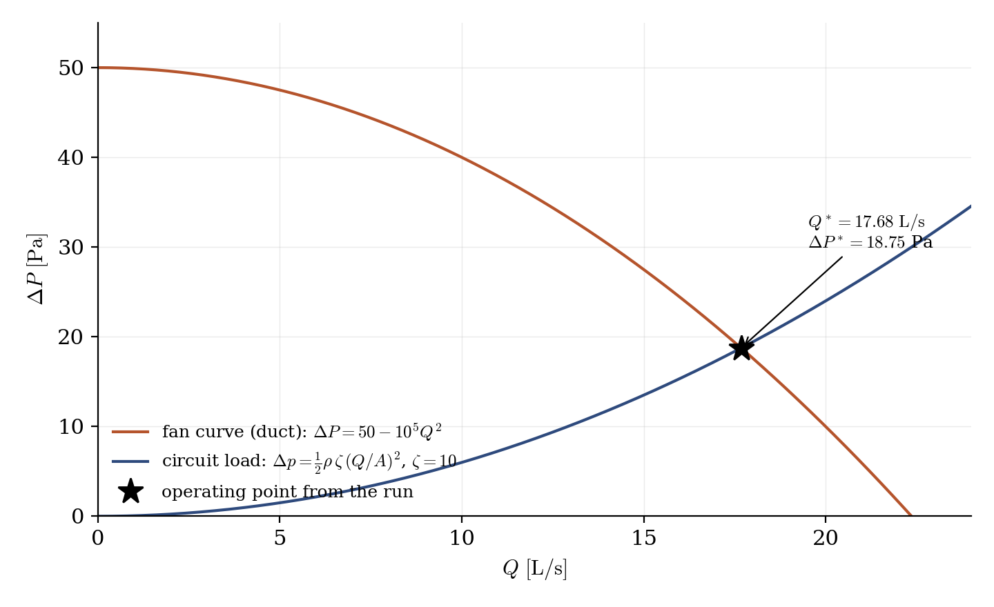
Fan curve and circuit load curve crossing at the operating point computed by the run.
Figure 2: the two curves and the computed operating point (star): $Q = 17.678$ L/s, on the intersection to five digits.

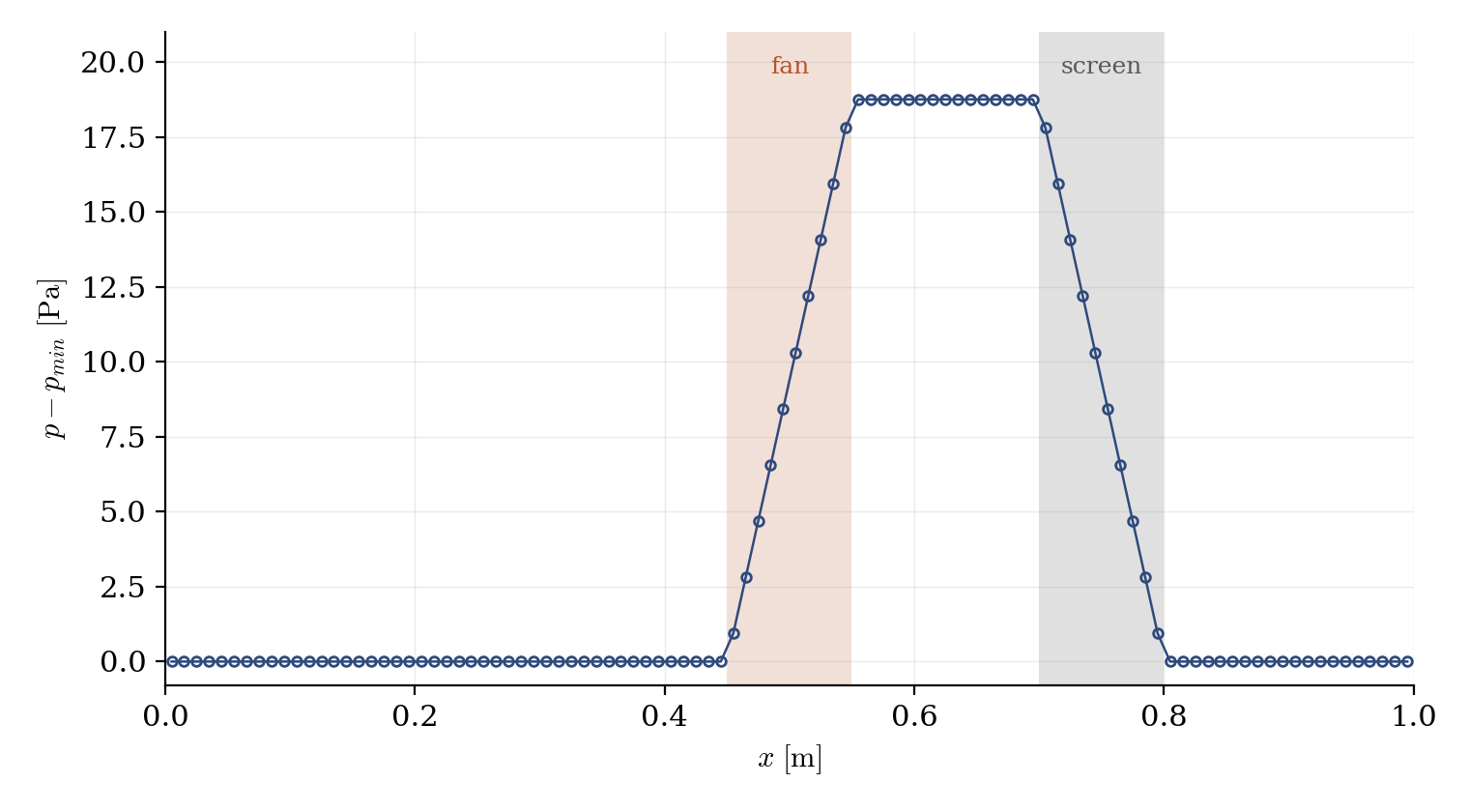
Pressure along the loop: rise across the fan, drop across the screen, flat elsewhere.
Figure 3: pressure along the loop: the fan raises exactly what the screen dissipates ($18.75$ Pa), with flat plateaus in the frictionless duct.

The equilibrium is exact to display precision: uniform plug velocity of $1.7678$ m/s, pressure span of $18.75$ Pa, flow rate on the predicted intersection to five digits.

Summary¶

This tutorial placed a virtual fan in a periodic duct loop, entirely from the GUI, and let the computation find the operating point of the fan curve against the circuit load: intersection reproduced to five digits. Two things to remember: use the pressure-jump mode (zero blade and hub radii) for an ideal actuator disk, and account for the thrust-conservation factor when the theoretical disk does not match the meshed section.

References¶

code_saturne documentation

Authors¶

Simvia - Questions, remarks and requests are welcome.