Supersonic Compression Ramp at Mach 2
A step-by-step tutorial for simulating the supersonic flow over a 10 degree compression ramp at \(M_1 = 2\) with the compressible module of code_saturne, and validating the attached oblique shock against the exact \(\theta\)-\(\beta\)-\(M\) relations.
Maintained by Simvia, part of the tutoriel-code_saturne collection.
Learning objectives
After completing this tutorial you will be able to:
- Compute a supersonic external flow with the compressible module (constant \(\gamma\)).
- Prescribe an inlet through its total conditions (\(P_t\), \(H_t\)) derived from the isentropic relations.
- Model slip walls for an inviscid flow with symmetry boundary conditions.
- Force the exact Euler limit with zero-valued GUI user laws for the viscosities and the conductivity.
- Validate a shock-capturing computation against the oblique shock relations.
Prerequisites
| Requirement | Detail |
|---|---|
| code_saturne | v9.1 |
| Background | Gas dynamics (oblique shocks); the Comp_Sod_Tube tutorial is the natural first step |
If code_saturne is not yet installed, build it from the official homepage, pull a ready-to-use Singularity image from the Open Simulation Center, or pull the Simvia Docker image before continuing.
Case files
Comp_Supersonic_Ramp/
├── CASE/
│   └── DATA/
│       └── setup.xml                        # pre-configured GUI case
├── MESH/
│   ├── ramp_10deg_shockref.msh              # mesh, refined along the shock (gmsh)
│   └── ramp_10deg_shockref.geo              # gmsh geometry and size-field source
├── FIGURES/                                 # figures used in this README
└── README.md
Physical model
The flow is steady, two-dimensional, supersonic and inviscid: the Euler equations for a perfect gas with \(\gamma = 1.4\) (see the Comp_Sod_Tube tutorial for the equation set). The inviscid limit is enforced exactly by GUI user laws setting the molecular viscosity, the volume viscosity and the thermal conductivity to zero (a GUI constant cannot be zero, but a user-law formula can; see the Comp_Sod_Tube tutorial).
A uniform stream at \(M_1 = 2\) meets a \(\theta = 10\) degree compression ramp. The exact solution is an attached oblique shock emanating from the ramp corner, whose angle \(\beta\) satisfies the \(\theta\)-\(\beta\)-\(M\) relation:
For \(M_1 = 2\), \(\theta = 10°\), \(\gamma = 1.4\) (weak solution): \(\beta = 39.3°\), and the normal-shock relations applied to \(M_{1n} = M_1 \sin\beta\) give the pressure ratio \(p_2/p_1 = 1.706\) and the downstream Mach number \(M_2 = 1.64\).
Inlet total conditions
The inlet is prescribed through its total pressure and total enthalpy (compressible inlet of type \(P_t\), \(H_t\)), computed from the target static state (\(p_1 = 101325\) Pa, \(T_1 = 287.5\) K, \(M_1 = 2\)) with the isentropic relations:
together with the velocity magnitude \(u_1 = M_1 \sqrt{\gamma R_s T_1} = 679.8\ \mathrm{m\,s^{-1}}\). Consistency matters here: these values are computed with \(c_p = 1004.85\ \mathrm{J\,kg^{-1}\,K^{-1}}\) (which gives exactly \(\gamma = c_p/(c_p - R_s) = 1.4\) with \(R_s = 287.06\)), and the same \(c_p\) is set in setup.xml. With this setup the computed upstream state comes out at \(M_1 = 2.0000\) and \(p_1 = 101328\) Pa.
Flow parameters
| Quantity | Symbol | Value | Source in setup.xml |
|---|---|---|---|
| Heat capacity ratio | \(\gamma\) | \(1.4\) | derived from specific_heat (\(1004.85\)) and reference_molar_mass |
| Upstream Mach number | \(M_1\) | \(2.0\) | via inlet total conditions |
| Upstream static state | \(p_1\), \(T_1\) | \(101325\) Pa, \(287.5\) K | targets of the \(P_t\)/\(H_t\) derivation |
| Ramp angle | \(\theta\) | \(10°\) | (geometry) |
| Inlet velocity | \(u_1\) | \(679.8\ \mathrm{m\,s^{-1}}\) | inlet/velocity_pressure/norm |
| Viscosity, conductivity | \(\mu\), \(\lambda\) | \(0\) (exact Euler limit) | user laws in fluid_properties |
Geometry and boundary conditions
The domain is a channel of height \(1.0\) m: a flat plate from \(x = 0\) to \(0.8\) m, followed by a \(10°\) ramp up to \(x = 1.8\) m. The height is chosen so that the oblique shock (\(\beta = 39.3°\) from the corner, reaching \(y = 0.82\) m at the outlet) leaves the domain through the outlet without touching the top boundary: the solution contains the single attached shock and nothing else. The mesh (MESH/ramp_10deg_shockref.msh, generated from the shipped ramp_10deg_shockref.geo with gmsh) is unstructured (recombined quadrangles, extruded one cell in \(z\)), with a background cell size of \(10\) mm refined to \(2.5\) mm in a band centered on the theoretical shock ray: since \(\beta\) is known in advance, the resolution is concentrated where the physics happens (\(\approx 29\,000\) cells, only \(1.6\) times a uniform \(10\) mm mesh, for a shock captured four times more sharply).
Since the flow is inviscid, the plate, the ramp and the upper boundary are slip walls, which are imposed with symmetry boundary conditions (zero normal velocity, no wall friction): this is the standard trick for Euler computations. The supersonic outlet requires no prescribed value.
| Boundary | Location | Nature | Prescribed value | Zone id |
|---|---|---|---|---|
INLET |
left (\(x=0\)) | Compressible inlet (\(P_t\), \(H_t\)) | \(792812.3\) Pa, \(520009.9\) J/kg, norm \(679.8\) m/s | 100 |
OUTLET |
right (\(x=1.8\)) | Supersonic outlet | (none) | 200 |
WALL |
plate + ramp | Slip wall (symmetry) | (none) | 500 |
UP |
top (\(y=1.0\)) | Slip wall (symmetry) | (none) | 300 |
SYM, SYM_TOP |
spanwise planes | Symmetry | (none) | 600, 601 |
Note on gmsh meshes: code_saturne selects boundary zones of a
.mshfile by the numeric physical tags (here 100, 200, 300, 500, 600, 601, set explicitly inramp_10deg_shockref.geo), not by the physical names.
Numerical setup
| Setting | Value | Rationale |
|---|---|---|
| Compressible algorithm | pressure-based, constant gamma |
code_saturne compressible module |
| Time-stepping | Variable time step, max CFL \(= 1\) | Pseudo-transient march to the steady state |
| Iterations | \(6000\) | Steady state reached well within this budget |
| Convection scheme | 1st-order upwind | Forced by the compressible module for all variables, whatever the GUI blending factor (cs_cf_model.cpp) |
| Gradients | Least-squares (extended) | Accuracy on the stretched mesh |
| Initialization | \(\mathbf{u} = (679.8, 0, 0)\), \(p = 101325\) Pa, \(T = 287.5\) K | Uniform upstream state |
| Viscosities, conductivity | \(0\) (user laws) | Exact Euler limit |
Running the simulation
The commands below start from the tutorial directory:
cd Comp_Supersonic_Ramp/
Option A: Graphical interface
code_saturne gui CASE/DATA/setup.xml &
The GUI opens the pre-configured setup.xml. Review the setup if you wish,
then launch the run with the gear (Run) button in the toolbar.
Option B: Command line
The command-line launcher is run from inside the case directory:
cd CASE

# serial
code_saturne run

# parallel (e.g. 4 MPI ranks)
code_saturne run --n 4
Each run creates a time-stamped directory CASE/RESU/<YYYYMMDD-HHMM>/ containing:
run_solver.log: solver log and residual history,postprocessing/: volume and boundary fields in EnSight Gold format (final state).
Results and verification
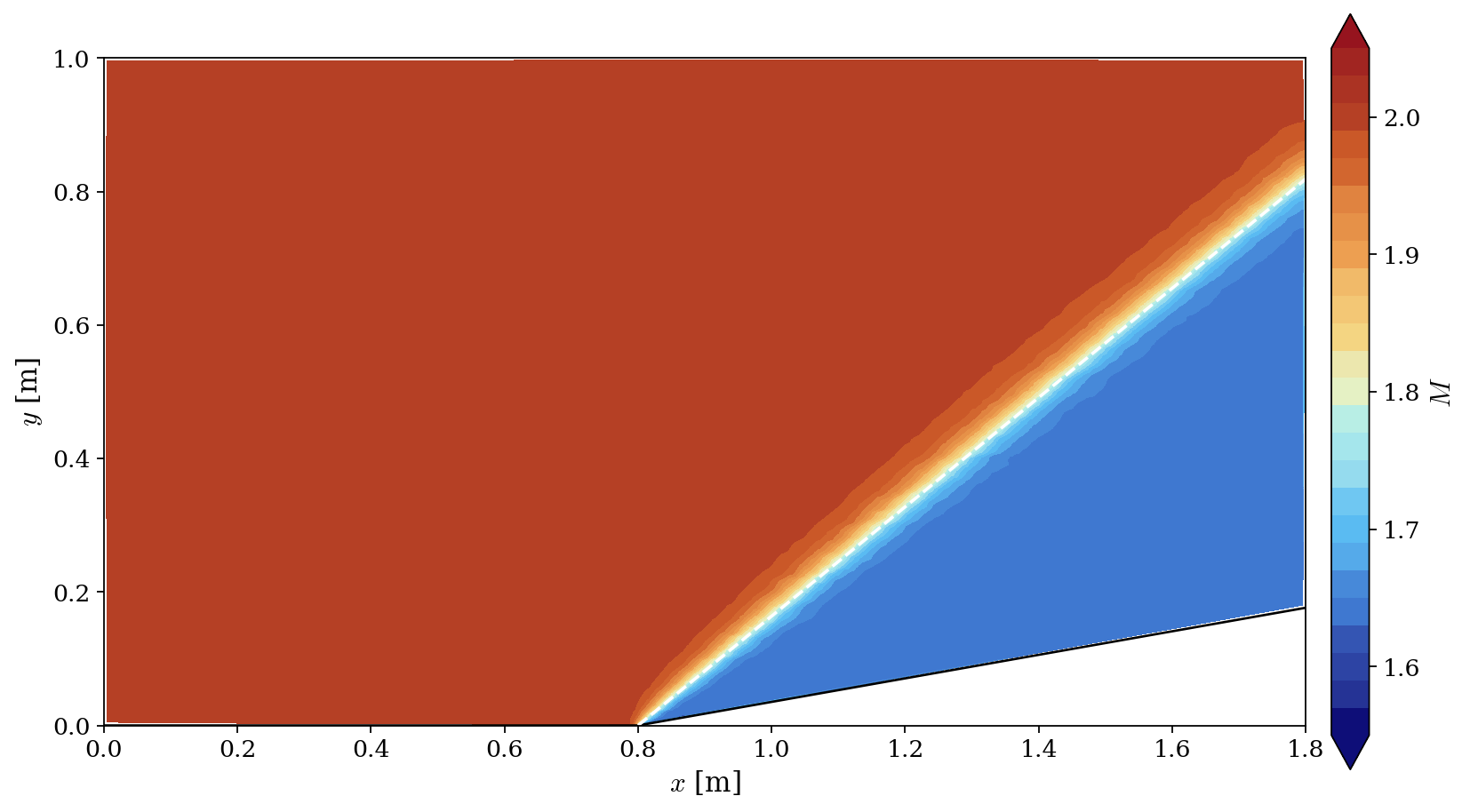
Figure 1: Mach number field at convergence. The white dashed line is the theoretical oblique shock ($\beta = 39.3°$) drawn from the ramp corner; the shock leaves the domain through the outlet without touching the top boundary.
The computed shock is attached to the corner (the measured shock line extrapolates to \(x_0 = 0.797\) m for a corner at \(0.8\) m) and follows the theoretical angle. The quantitative comparison against the oblique shock relations, using the measured upstream state (\(M_1 = 2.0000\)):
| Quantity | code_saturne | Oblique shock theory | Error |
|---|---|---|---|
| Shock angle \(\beta\) | \(39.4°\) | \(39.3°\) | \(0.2\%\) |
| Pressure ratio \(p_2/p_1\) | \(1.707\) | \(1.706\) | \(0.01\%\) |
| Downstream Mach \(M_2\) | \(1.638\) | \(1.641\) | \(0.2\%\) |
The shock angle is measured by locating, on each vertical line between \(x = 0.90\) and \(1.60\) m, the crossing of the mid-jump isobar \(p = (p_1 + p_2)/2\), and fitting a straight line through these points (\(R^2 = 0.99999\)); the post-shock values are averaged between the ramp surface and the shock. The captured shock keeps a finite numerical thickness: the 1st-order upwind convection scheme diffuses the discontinuity over a few cells, which is why the mesh is refined along the shock. Away from this transition the upstream state remains strictly uniform at \(M = 2.0000\).
Summary
This tutorial computed the \(M_1 = 2\) flow over a \(10°\) compression ramp with the compressible module of code_saturne: inlet prescribed by its total conditions derived from the isentropic relations, slip walls imposed as symmetries, and exact Euler limit enforced by zero user laws.
References
- J.D. Anderson. Modern Compressible Flow: With Historical Perspective, 3rd edition, McGraw-Hill, 2003 (chapter 4, oblique shocks).
- NACA Report 1135, Equations, Tables and Charts for Compressible Flow, 1953.
- code_saturne documentation
Authors
Simvia - Questions, remarks and requests are welcome.