Turbulent Bend with Wall Functions (RANS Model Comparison)
A step-by-step tutorial for RANS turbulence modelling with wall functions in code_saturne, on the reference experiment of Sudo et al. (1998): the steady turbulent flow through a circular 90 degree pipe bend. The bend generates strong curvature-driven secondary flow and a low-velocity region near the inner wall, a demanding test where turbulence closures disagree. Two models are compared on the same mesh and the same near-wall treatment, and confronted with the experimental data and a reference LES: the tutorial's purpose is the model comparison workflow, the validation being the bonus.
Maintained by Simvia, part of the tutoriel-code_saturne collection.
Learning objectives
After completing this tutorial you will be able to:
- Set up a steady incompressible RANS simulation on an imported 3D mesh, driven to steady state with local (pseudo) time-stepping and SIMPLEC.
- Run the same case with two turbulence models (k-\(\omega\) SST and Rij-EBRSM) by changing a single GUI setting, and compare them cleanly (identical mesh, numerics and wall treatment).
- Understand and justify the all-\(y^+\) wall function from the actual near-wall \(y^+\) of the run.
- Post-process a bend flow: cross-section velocity contours, symmetry-line profiles, and comparison against experimental and LES data.
Prerequisites
| Requirement | Detail |
|---|---|
| code_saturne | v9.1 |
| Tutorial | Inc_Turbulent_Plate (RANS basics and wall functions) |
If code_saturne is not yet installed, build it from the official homepage, pull a ready-to-use Singularity image from the Open Simulation Center, or pull the Simvia Docker image before continuing.
Case files
Inc_Turbulent_Bend_Wallfunctions/
├── CASE_kwSST/
│   └── DATA/setup.xml     # k-omega SST
├── CASE_RSM/
│   └── DATA/setup.xml     # Rij-EBRSM; identical but for the turbulence model
├── MESH/
│   └── sudo_coarse.msh    # 90-degree bend, half pipe (Git LFS)
├── FIGURES/               # figures used in this README
└── README.md
The two
setup.xmldiffer only by the turbulence model (and its variables): same mesh, same boundary conditions, same numerics, same all-\(y^+\) wall function. Diff them to see it. The mesh is tracked with Git LFS.
Physical model
The flow is steady, incompressible and fully turbulent, governed by the Reynolds-Averaged Navier-Stokes equations. The turbulent stress is closed with two models compared here:
- k-\(\omega\) SST (Menter): a two-equation eddy-viscosity model, isotropic, robust in adverse pressure gradients;
- Rij-EBRSM: a seven-equation Reynolds-stress model that transports the stress tensor itself, capturing the anisotropy that curvature-driven secondary flow produces.
The bend is precisely the flow where these differ: the mean strain rotates through the curve and the turbulence becomes strongly anisotropic, which an eddy-viscosity model cannot represent by construction.
Flow parameters (Sudo et al. 1998)
| Quantity | Symbol | Value | Source |
|---|---|---|---|
| Pipe diameter | \(D = 2a\) | \(0.104\) m | mesh |
| Bend curvature radius | \(R_c\) | \(0.208\) m (\(R_c/a = 4\)) | mesh |
| Bulk velocity | \(W_a\) | \(8.7\) m/s | inlet |
| Density | \(\rho\) | \(1.185\ \mathrm{kg\,m^{-3}}\) | fluid_properties |
| Dynamic viscosity | \(\mu\) | \(1.785\times10^{-5}\ \mathrm{Pa\,s}\) | fluid_properties |
| Reynolds number | \(Re = \rho W_a D/\mu\) | \(\approx 6\times10^{4}\) | derived |
Geometry and boundary conditions
A 90 degree bend of diameter \(D = 0.104\) m and curvature radius \(R_c = 2D\), with a straight upstream tangent of \(5D\) and a downstream tangent of \(10D\). Only the upper half of the pipe is meshed, with a symmetry plane on the bend mid-plane (\(y = 0\)): this halves the cost. Note that this is not a 2D computation: the bend drives a genuine three-dimensional secondary flow (a pair of counter-rotating Dean vortices), and the symmetry plane only exploits the top/bottom mirror symmetry of that flow.
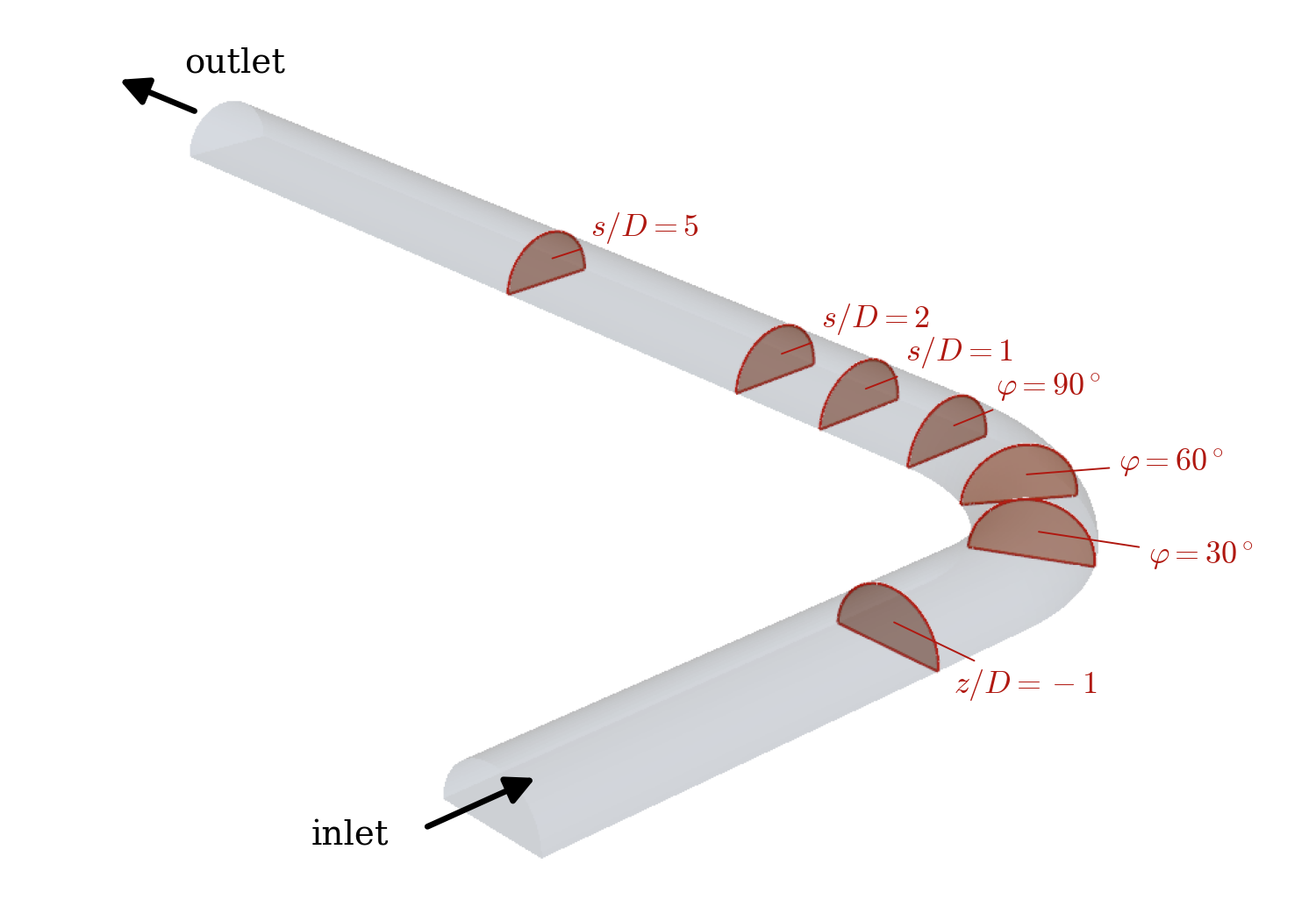
Figure 1: the computational domain (isometric view, transparent walls). Flow enters the $5D$ upstream tangent, turns through the $90°$ bend ($R_c = 2D$), and leaves through the $10D$ downstream tangent; only the upper half of the pipe is meshed (flat symmetry plane visible underneath). The half-disks locate the cross-section stations used below: $z/D = -1$ upstream, $\varphi = 30/60/90°$ in the bend, and $s/D = 1/2/5$ downstream.
| Boundary | Nature | Prescribed |
|---|---|---|
inlet |
inlet | uniform \(W_a = 8.7\) m/s, turbulence from hydraulic diameter |
outlet |
outlet | \(p = 0\) |
wall_1, wall_bend, wall_2 |
no-slip wall + all-\(y^+\) | \(\mathbf{u} = 0\) |
symmetry_1, symmetry_bend, symmetry_2 |
symmetry | mid-plane |
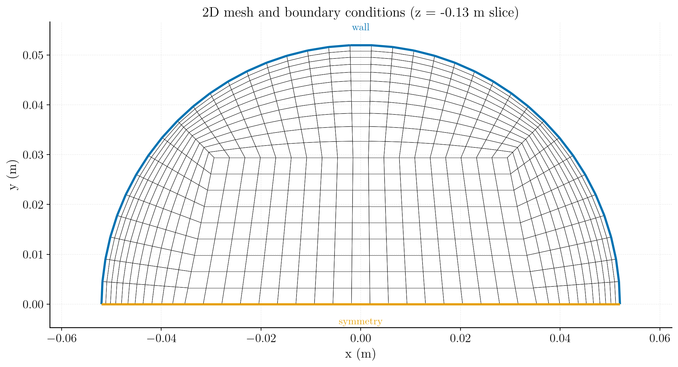
Figure 2: the cross-section mesh (half pipe, O-grid topology). The curved outer boundary is a no-slip wall (blue), the flat bottom is the symmetry mid-plane (orange). This section is swept along the upstream tangent, through the bend and along the downstream tangent.
Two honest limitations of this coarse setup, relative to the experiment: the upstream tangent is \(5D\) (the experiment has \(100D\), giving a fully-developed inlet profile), and the inlet here is uniform rather than a developed pipe profile. The bend dynamics dominate the comparison, but these choices explain part of the departure from the measurements.
Numerical setup
| Setting | Value | Rationale |
|---|---|---|
| Coupling | SIMPLEC | robust steady segregated coupling |
| Time-stepping | local (pseudo) time step | accelerates convergence to steady state |
| Wall function | all \(y^+\) (2-scale) on both models | see below |
| Turbulence | k-\(\omega\) SST / Rij-EBRSM | the compared closures |
| Iterations | to residual plateau (a few hundred to ~1000) | steady state |
Why the all-\(y^+\) wall function
On this coarse mesh the first-cell \(y^+\) does not sit cleanly in the logarithmic layer (\(y^+ > 30\)) where the standard log-law wall function is valid, nor in the viscous sublayer (\(y^+ \approx 1\)) required by a low-Reynolds model. Instead it falls almost entirely in the buffer layer (\(5 < y^+ < 30\)), and varies along the walls with the acceleration and separation. The all-\(y^+\) treatment (Menter's 2-scale blending) is designed exactly for this range, which is why it is used, and used identically on both models so the comparison isolates the turbulence closure alone.
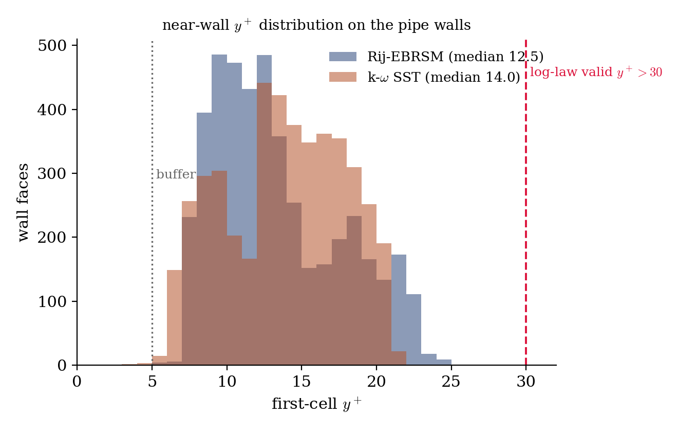
Figure 3: distribution of the first-cell $y^+$ over the pipe walls for both models. Every wall face lies below the $y^+ = 30$ log-law validity threshold, mostly in the buffer layer ($5 < y^+ < 30$): the regime the all-$y^+$ treatment is built for.
Running the simulation
The commands below start from the tutorial directory. Run each case (parallel recommended, ~70k cells):
cd CASE_kwSST
code_saturne run --n 4

cd ../CASE_RSM
code_saturne run --n 4
To switch model in the GUI instead, open either setup.xml and change the model under Thermophysical models → Turbulence. Convergence is reached when the residuals plateau (a few hundred iterations); the monitoring probe and residuals.csv track it.
Results and verification
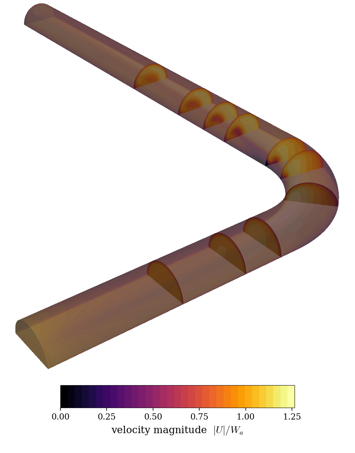
Figure 4: three-dimensional overview (Rij-EBRSM) with cross-section slices coloured by the velocity magnitude normalized by the bulk velocity, $|U|/W_a$. The fast fluid hugs the inner wall entering the bend and the secondary flow redistributes it downstream: the signature of a strongly curved pipe.
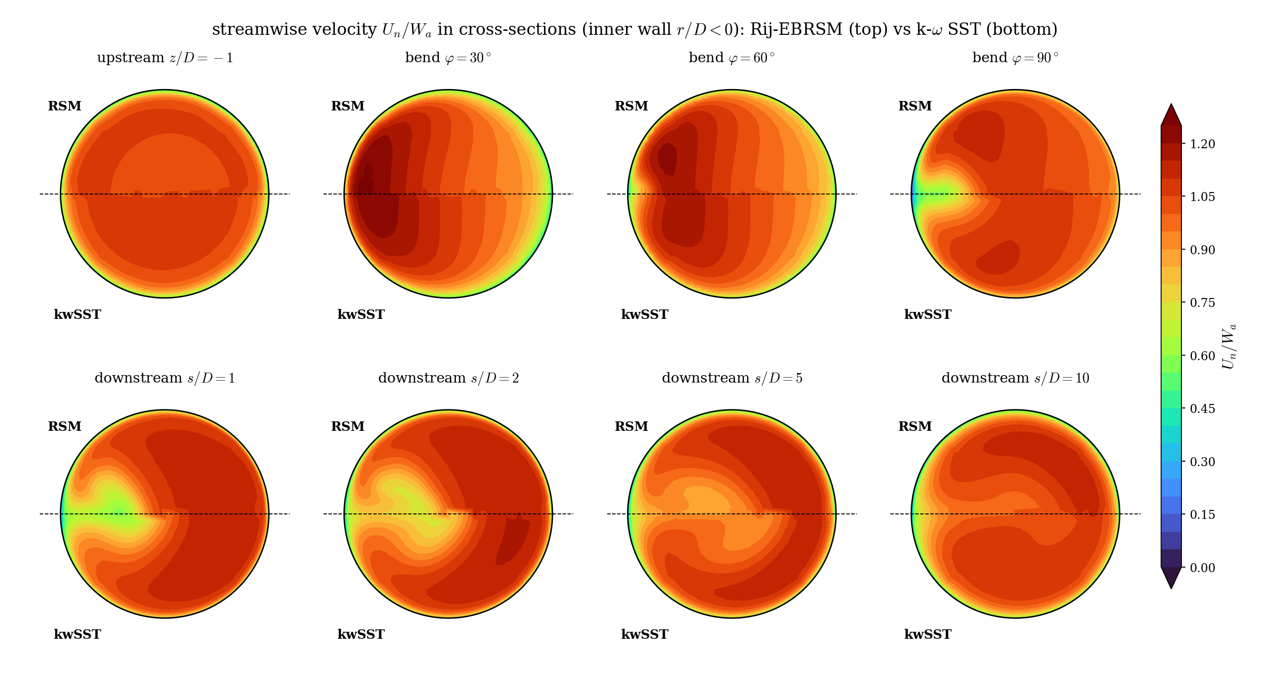
Figure 5: streamwise velocity in the eight cross-sections located in Figure 1 (Rij-EBRSM top half, k-$\omega$ SST bottom half of each disk). The fast fluid moves to the inner wall entering the bend, a low-velocity depression forms near the inner wall by $\varphi = 90°$, and the secondary flow smears it into the characteristic two-lobe pattern downstream, fading by $s/D = 10$. The two models tell the same qualitative story with visible quantitative differences.
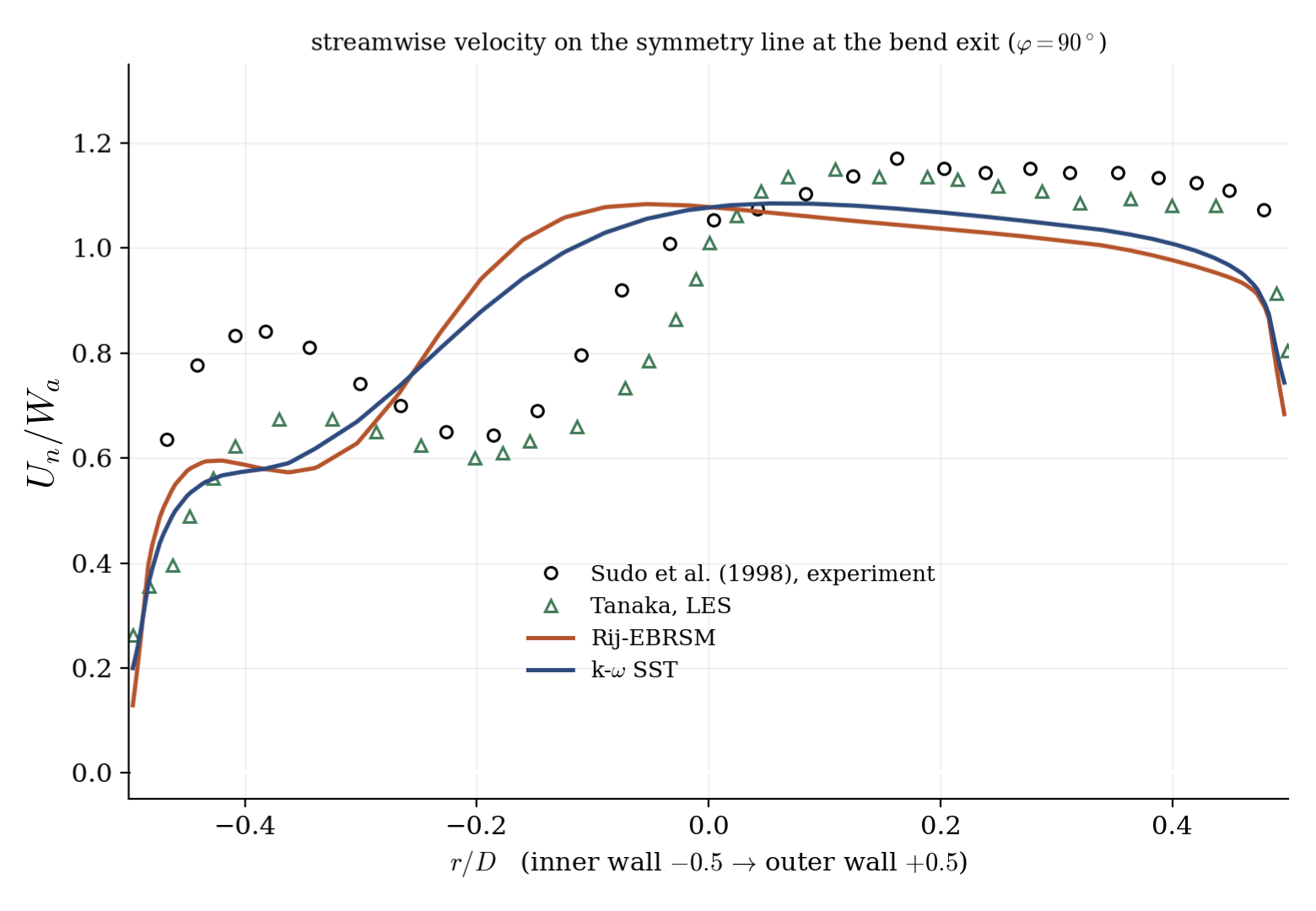
Figure 6: streamwise velocity on the symmetry line at the bend exit ($\varphi = 90°$), against Sudo et al.'s experiment and Tanaka's LES. Both RANS models reproduce the shape (inner-wall depression, core acceleration) but under-predict the inner-wall velocity and stay below the measurements toward the outer wall.
The comparison is honest about what RANS captures here. Both models give the correct qualitative profile at \(\varphi = 90°\) and are close to each other, the Rij-EBRSM being slightly fuller near the inner wall. Neither reproduces the detailed inner-wall velocity distribution measured by Sudo (the shoulder-and-dip structure driven by the secondary flow), and both sit below the experiment and the LES across much of the section. This is the expected behaviour of steady RANS on a strongly curved bend, and it is compounded here by the coarse mesh, the short \(5D\) upstream tangent and the uniform inlet.
Summary
This tutorial ran the Sudo 90 degree bend with two RANS closures (k-\(\omega\) SST and Rij-EBRSM) sharing one mesh, one set of numerics and one all-\(y^+\) wall treatment, so the comparison isolates the turbulence model. The near-wall \(y^+\) justifies the all-\(y^+\) choice (buffer layer throughout). Both models capture the bend physics qualitatively (inner-wall depression, secondary-flow two-lobe pattern) and are confronted with experiment and LES; the quantitative gaps are stated honestly and traced to the closures and the coarse, short-inlet setup.
References
- K. Sudo, M. Sumida, H. Hibara. Experimental investigation on turbulent flow in a circular-sectioned 90-degree bend, Experiments in Fluids 25, 42-49, 1998.
- code_saturne documentation
Authors
Simvia, from an initial setup by Abderrazak (Simvia intern). Questions, remarks and requests are welcome.