Joule Heating of a Conducting Bar

Browse this case on GitHub

A step-by-step tutorial for the Joule effect module of code_saturne: a static conducting bar carries a current between two electrodes, and the Joule dissipation heats it against its cooled walls. Everything has a closed form: the potential is linear, the total power is \(P = UI\), and the steady temperature profile is a parabola. The case is the entry point of the electric module, and documents the three user-file requirements of its Joule variant.

Maintained by Simvia, part of the tutoriel-code_saturne collection.

Learning objectives

After completing this tutorial you will be able to:

1. Enable the Joule effect model (real potential, AC/DC) and understand what the module solves.
2. Provide the electrical conductivity (the diffusivity of the potential) and the temperature-enthalpy law in cs_user_physical_properties.cpp.
3. Impose the electrode potentials in cs_user_boundary_conditions.cpp (required by a GUI limitation of this version).
4. Verify the computation against the exact solution (potential, power, current, temperature parabola).

Prerequisites

Requirement	Detail
code_saturne	v9.1
Background	Basic electrokinetics (\(\mathbf{j} = \sigma \mathbf{E}\), Joule dissipation)

If code_saturne is not yet installed, build it from the official homepage, pull a ready-to-use Singularity image from the Open Simulation Center, or pull the Simvia Docker image before continuing.

Case files

Elec_Joule_Bar/
├── CASE/
│   ├── DATA/
│   │   └── setup.xml                        # pre-configured GUI case
│   └── SRC/
│       ├── cs_user_physical_properties.cpp  # sigma + T(H) law (MANDATORY)
│       └── cs_user_boundary_conditions.cpp  # electrode potentials (MANDATORY)
├── FIGURES/                                 # figures used in this README
└── README.md

There is no MESH directory: the mesh is generated at run time by the built-in cartesian mesher.

Physical model

The Joule module solves a Poisson equation for the electric potential, with the electrical conductivity as diffusivity, alongside the flow and energy equations:

\[ \nabla \cdot (\sigma \nabla \phi) = 0, \qquad \mathbf{j} = -\sigma \nabla \phi, \qquad q_J = \sigma\, |\nabla \phi|^2 \]

and injects the volumetric Joule power \(q_J\) into the enthalpy equation (the thermal variable imposed by the module). The fluid here is kept static (no gravity, closed walls): it behaves as a solid conductor, and the case reduces to electrokinetics plus heat conduction.

With a potential difference \(U\) over the length \(L\) of a homogeneous bar, everything is closed-form:

\[ E = U/L, \qquad q_J = \sigma E^2, \qquad I = \sigma E A, \qquad P = UI = q_J\, V \]

and at steady state, the uniformly heated bar cooled by its two lateral walls (gap \(h\)) takes the parabolic profile

\[ T(y) = T_w + \frac{q_J}{2\lambda}\, y\, (h - y), \qquad \Delta T_{max} = \frac{q_J h^2}{8\lambda} \]

The three user-file requirements of the Joule variant

The electric-arc variant of the module reads its plasma properties from a data file; the Joule variant delegates them to user code (its industrial use, glass furnaces, involves strongly temperature-dependent material laws). Three things must be provided:

1. The electrical conductivity (\(\sigma\), here \(100\ \mathrm{S/m}\) constant): it is the diffusivity field of the potential, filled in cs_user_physical_properties.cpp. Any \(\sigma(T)\) law fits in the same loop.
2. The temperature-enthalpy conversion: the module only performs it for electric arcs (from tabulated plasma properties); for the Joule variant the temperature property field must be filled by the user. With a constant \(c_p\), simply \(T = H/c_p\).
3. The electrode potentials: the GUI accepts Dirichlet values for elec_pot_r, but in this version its reader only applies the joule_effect variable boundary conditions when the electric arc model is active: for the pure Joule model they are silently ignored (the potential stays at zero and nothing heats). cs_user_boundary_conditions.cpp imposes them directly on the electrode zones with cs_equation_add_bc_by_value.

One more GUI quirk worth knowing: enabling the electric model converts the constant fluid properties to user law mode; check that the density formula carries your value and not the default rho0 reference.

Flow parameters

Quantity	Symbol	Value	Source
Bar	\(L \times h \times e\)	\(100 \times 20 \times 5\) mm	mesh_cartesian
Electrical conductivity	\(\sigma\)	\(100\ \mathrm{S/m}\)	cs_user_physical_properties.cpp
Potential difference	\(U\)	\(10\) V	cs_user_boundary_conditions.cpp
Material	\(\rho\), \(c_p\), \(\lambda\)	\(1000\), \(100\), \(10\) (SI)	fluid_properties
Wall temperature	\(T_w\)	\(300\) K (\(H_w = c_p T_w = 30000\ \mathrm{J/kg}\))	Cooled wall BC
Joule power	\(q_J\), \(P\)	\(10^6\ \mathrm{W/m^3}\), \(10\) W	derived
Current	\(I\)	\(1\) A	derived
Expected overheat	\(\Delta T_{max}\)	\(5\) K	derived
Time	\(\Delta t\), \(N\)	\(10^{-2}\) s, \(500\) steps (\(5\) diffusion times)	time_parameters

Geometry and boundary conditions

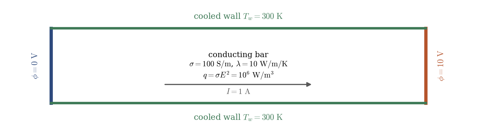
Figure 1: the bar. Electrodes at the ends (potential Dirichlet, adiabatic in temperature), cooled lateral walls (fixed temperature, electrically insulated), symmetry on the spanwise planes.

Boundary	Location	Electric	Thermal
Electrode0	\(x = 0\)	\(\phi = 0\) V (user routine)	adiabatic
Electrode1	\(x = L\)	\(\phi = 10\) V (user routine)	adiabatic
Cooled	\(y = 0\), \(y = h\)	insulated (zero flux)	\(T_w = 300\) K (enthalpy Dirichlet)
Sym	spanwise planes	Symmetry	Symmetry

Numerical setup

Setting	Value	Rationale
Electric model	Joule, AC/DC (real potential only)	DC conduction
Potential scaling	off	The potential difference is imposed directly
Thermal variable	enthalpy (imposed by the module)	BC values are enthalpies: \(H = c_p T\)
Flow	static (no gravity, closed box)	The "fluid" is a solid conductor
Time-stepping	\(\Delta t = 10^{-2}\) s, \(500\) steps	\(\approx 5\) thermal diffusion times to steady state

Running the simulation

The commands below start from the tutorial directory:

cd Elec_Joule_Bar/

Option A: Graphical interface

code_saturne gui CASE/DATA/setup.xml &

The GUI opens the pre-configured setup.xml. Review the setup if you wish, then launch the run with the gear (Run) button in the toolbar.

Option B: Command line

The command-line launcher is run from inside the case directory:

cd CASE

# serial (a few seconds)
code_saturne run

The two user routines are compiled automatically at the beginning of the run.

Results

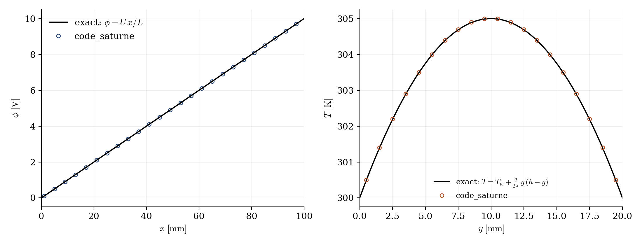
Figure 2: left, electric potential along the bar: linear at $100.0000$ V/m (deviation from linearity below $10^{-6}$ V). Right, temperature across the bar at mid-length: the exact parabola, with $\Delta T_{max} = 5.000$ K (deviation $\approx 0.01$ K, the discretization of the wall gradient).

The three integral checks land on the exact values: total Joule power \(P = 10.00000\) W (\(= UI\)), current \(I = 1.00000\) A (\(= \sigma E A\)), and uniform dissipation \(q_J = 10^6\ \mathrm{W/m^3}\) (\(= \sigma E^2\)). As in the other exact-solution cases of this collection, the point is not the agreement itself (the module discretizes these very formulas) but what it certifies: the chain electrode potentials → potential field → current → dissipation → enthalpy source → temperature is wired correctly, with every user-provided piece in place.

Summary

This tutorial set up the Joule variant of the electric module on its simplest possible case: a static conducting bar between two electrodes. The module solves the potential with \(\sigma\) as diffusivity and feeds the Joule power to the enthalpy; the user provides the conductivity, the temperature-enthalpy law, and (owing to a GUI limitation of this version) the electrode potential boundary conditions. Potential slope, current, power and the steady temperature parabola all match the closed-form solution.

References

• J.A. Stratton. Electromagnetic Theory, McGraw-Hill, 1941.
• code_saturne documentation

Authors

Simvia - Questions, remarks and requests are welcome.