Imposed Power (Electric Potential Scaling)

Browse this case on GitHub

A step-by-step tutorial for the imposed-power mode of the Joule module of code_saturne: instead of prescribing the electrode potentials, the operator prescribes the dissipated power, and the module rescales the potentials automatically at every time step: this is how electric furnaces are actually driven. On the bar of Elec_Joule_Bar, imposing \(P = 40\) W must yield \(U = \sqrt{PR} = 20\) V exactly. The case also documents (and fixes, through the official user hook) a convergence flaw of the built-in scaling iteration for the Joule variant.

Maintained by Simvia, part of the tutoriel-code_saturne collection.

Learning objectives

After completing this tutorial you will be able to:

1. Drive a Joule computation by imposed power (variable_scaling, imposed_power): the potential boundary conditions become a shape, whose amplitude the module finds.
2. Write rescaling-aware potential boundary conditions (a dof function multiplying the seed by the module's cumulative coefficient coejou).
3. Use the official hook cs_user_scaling_elec to impose your own regulation law, and understand why the built-in Joule power iteration cycles instead of converging.

Prerequisites

Requirement	Detail
code_saturne	v9.1
Case	Elec_Joule_Bar (the same bar with imposed potentials, and the user-file requirements of the Joule variant)

If code_saturne is not yet installed, build it from the official homepage, pull a ready-to-use Singularity image from the Open Simulation Center, or pull the Simvia Docker image before continuing.

Case files

Elec_Imposed_Power/
├── CASE/
│   ├── DATA/
│   │   └── setup.xml                        # Elec_Joule_Bar + scaling on, imposed_power 40
│   └── SRC/
│       ├── cs_user_physical_properties.cpp  # sigma + T(H) law (as Elec_Joule_Bar)
│       ├── cs_user_boundary_conditions.cpp  # SEED potentials, rescaled by coejou
│       └── cs_user_electric_scaling.cpp     # square-root correction of the scaling
├── FIGURES/                                 # figures used in this README
└── README.md

Physical model

The bar is that of Elec_Joule_Bar (\(R = L/(\sigma A) = 10\ \Omega\)). With the potential scaling enabled (ielcor = 1), the module compares at each step the dissipated power \(P = \int \sigma |\nabla \phi|^2\,dV\) to the imposed one and multiplies the potential (field and boundary values, through the cumulative coefficient coejou) by a correction factor. At convergence:

\[ U = \sqrt{P\,R} = \sqrt{40 \times 10} = 20\ \mathrm{V}, \qquad I = U/R = 2\ \mathrm{A}, \qquad q_J = P/V = 4 \times 10^6\ \mathrm{W/m^3} \]

and the steady thermal parabola scales accordingly: \(\Delta T_{max} = q_J h^2 / (8\lambda) = 20\) K.

Boundary conditions become a shape

With the scaling active, the electrode Dirichlet values are only a seed: the module stretches them by coejou until the power matches. Two consequences for the user files:

• the potential boundary condition must be evaluated through a function that multiplies the seed by cs_glob_elec_option->coejou at every evaluation (a cs_dof_func_t registered with cs_equation_add_bc_by_dof_func), otherwise the rescaling never reaches the boundary. This mirrors what the GUI does for the arc model;
• the seed value is arbitrary (here \(10\) V): the converged coejou simply becomes \(U/\mathrm{seed} = 2.0\).

The scaling iteration, and its fix

The built-in Joule rescaling multiplies the potential by the power ratio \(P_{imp}/P_n\). Since \(P \propto U^2\), this over-corrects: the iteration \(U_{n+1} = U^{*2}/U_n\) has an unstable fixed point, and the computation cycles forever between two values (a period-2 oscillation, clearly visible in the log and in Figure 1) instead of converging: the potential difference never settles and the power bounces around the target. The correct factor is the square root of the power ratio, and the module provides the official place to impose it: the hook cs_user_scaling_elec, called right after the built-in rescaling at every step. The shipped cs_user_electric_scaling.cpp recomputes the dissipated power and applies \(k = \sqrt{P_{imp}/P}\) to the potential, coejou and the Joule power: the linear potential equation then lands exactly on the imposed power in a single step.

Flow parameters

Quantity	Symbol	Value	Source
Imposed power	\(P\)	\(40\) W	imposed_power (GUI)
Bar resistance	\(R\)	\(10\ \Omega\) (\(\sigma = 100\ \mathrm{S/m}\))	cs_user_physical_properties.cpp
Seed potential		\(10\) V (arbitrary)	cs_user_boundary_conditions.cpp
Expected converged state	\(U\), \(I\), coejou	\(20\) V, \(2\) A, \(2.0\)	derived
Expected overheat	\(\Delta T_{max}\)	\(20\) K	derived
Bar, material, mesh, time		as in Elec_Joule_Bar	setup.xml

Geometry and boundary conditions

Identical to Elec_Joule_Bar: electrodes at the ends (grounded / powered), cooled lateral walls at \(300\) K, symmetry on the spanwise planes.

Numerical setup

As in Elec_Joule_Bar, plus:

Setting	Value	Rationale
Potential scaling	on (variable_scaling)	Imposed-power drive
Imposed power	\(40\) W	The regulation target
User scaling law	\(k = \sqrt{P_{imp}/P}\)	cs_user_electric_scaling.cpp (see above)

Running the simulation

The commands below start from the tutorial directory:

cd Elec_Imposed_Power/

Option A: Graphical interface

code_saturne gui CASE/DATA/setup.xml &

The GUI opens the pre-configured setup.xml. Review the setup if you wish, then launch the run with the gear (Run) button in the toolbar.

Option B: Command line

The command-line launcher is run from inside the case directory:

cd CASE

# serial (a few seconds)
code_saturne run

The three user routines are compiled automatically at the beginning of the run. The scaling history is printed at every step in run_solver.log (imposed power / sum(jE) lines).

Results

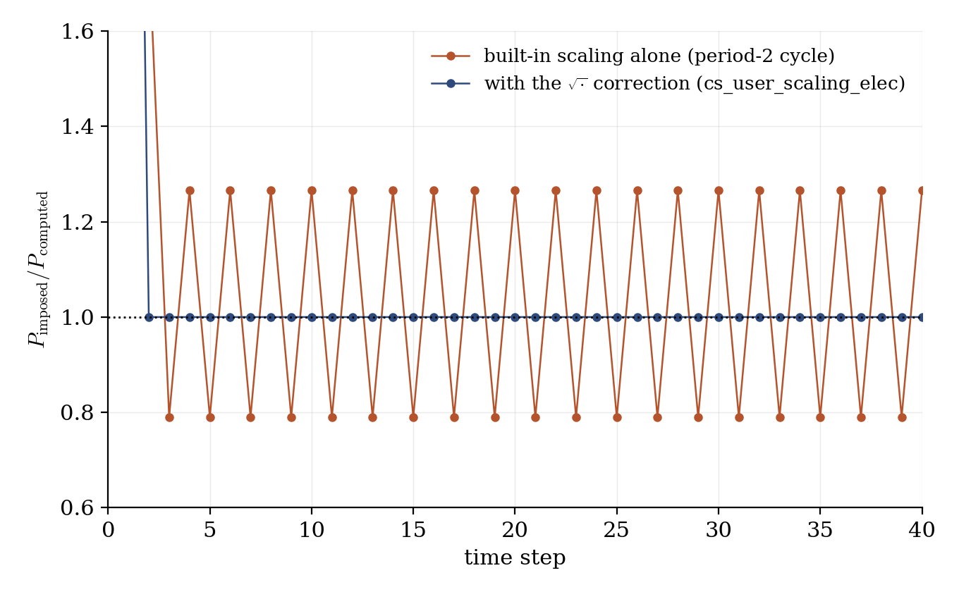
Figure 1: the regulation at work: ratio of imposed to computed power at each step. With the built-in scaling alone, the iteration locks into the predicted period-2 cycle ($0.79 \leftrightarrow 1.27$) and never converges; with the square-root correction in cs_user_scaling_elec, the ratio is $1.00000$ from the second step onward.

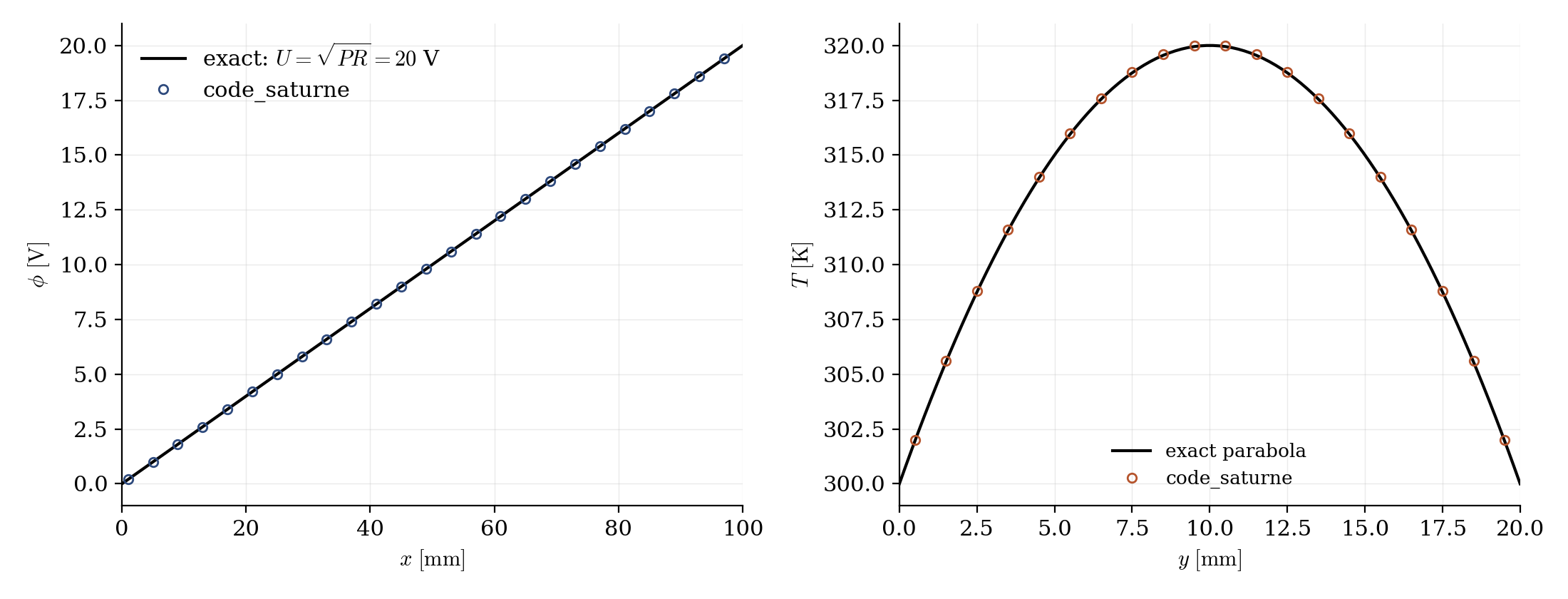
Figure 2: converged state. The potential found by the regulation spans $U = 20.00$ V ($E = 200.0000\ \mathrm{V/m}$), i.e. $\mathrm{coejou} = 2.0$ from the $10$ V seed; the thermal parabola reaches $T_{max} = 320.0000$ K. Computed integrals: $I = 2.00000$ A, $P = 40.00000$ W.

Summary

This tutorial drove the Joule bar by imposed power: the electrode potentials become a seed shape rescaled by the module (evaluated through a coejou-aware boundary function), and the regulation finds \(U = \sqrt{PR} = 20\) V exactly. The built-in Joule scaling iteration is shown to cycle rather than converge (it applies the power ratio where its square root is needed), and the official cs_user_scaling_elec hook fixes it in one line: a useful pattern for any custom furnace regulation law.

References

• code_saturne documentation

Authors

Simvia - Questions, remarks and requests are welcome.