Turbulent Species Transport in a Mixing Channel
A step-by-step tutorial for simulating the steady, incompressible, turbulent flow in a mixing channel with passive species transport, using code_saturne. Two streams of different composition merge at a T-junction and mix along the downstream duct.
Maintained by Simvia, part of the tutoriel-code_saturne collection.
Learning objectives
After completing this tutorial you will be able to:
- Set up a steady, incompressible turbulent (k-\(\omega\) SST) simulation in code_saturne from the GUI.
- Add passive species (user scalars) with inlet Dirichlet and zero-flux boundary conditions.
- Apply the N-species closure: solve N-1 transport equations and deduce the last mass fraction.
- Drive a steady solution with local (pseudo) time-stepping and the SIMPLEC coupling.
- Verify the computed mixing against an analytic species mass balance.
- Run the case in serial or parallel and locate the solver outputs (log, probes, EnSight fields).
Limitations
Mixture-dependent fluid properties are not available at this stage: the density and viscosity do not depend on the local composition, and a single constant mass diffusion coefficient is applied to all species. The species are therefore passive scalars.
Prerequisites
| Requirement | Detail |
|---|---|
| code_saturne | v9.1 |
| Background | Basic notions of incompressible turbulent flow and mass transfer theory |
| Case | Inc_Turbulent_Plate |
If code_saturne is not yet installed, build it from the official homepage, pull a ready-to-use Singularity image from the Open Simulation Center, or pull the Simvia Docker image before continuing.
Case files
Inc_Species_Transport/
├── CASE/
│   └── DATA/
│       └── setup.xml          # pre-configured GUI case
├── MESH/
│   └── primitiveVenturi.msh
├── FIGURES/                   # figures used in this README
└── README.md
Physical model
The flow is steady, incompressible, isothermal and turbulent (RANS with the k-\(\omega\) SST model). The mixture contains three species A, B and C with identical physical properties, so the composition does not influence the flow: the mass fractions are passive scalars. Following the standard closure, only N-1 = 2 transport equations are solved (for \(Y_A\) and \(Y_B\)), and the third mass fraction is deduced from
The solver marches the following system to steady state:
where the turbulent viscosity \(\mu_t\) is given by the k-\(\omega\) SST model (two additional transport equations for \(k\) and \(\omega\), see the code_saturne theory guide), \(D\) is the molecular mass diffusivity and \(\sigma_t = 1\) is the turbulent Schmidt number (code_saturne default).
Note on units: the species diffusion coefficient entered in the GUI is the kinematic diffusivity \(D\) in m²/s; code_saturne converts it internally to the dynamic diffusivity \(\rho D\). When setting it through
cs_user_parameters.cppinstead, the dynamic value is expected.
Flow parameters
| Quantity | Symbol | Value | Source in setup.xml |
|---|---|---|---|
| Density | \(\rho\) | \(1.1766\ \mathrm{kg\,m^{-3}}\) | physical_properties/density |
| Dynamic viscosity | \(\mu\) | \(1.716 \times 10^{-5}\ \mathrm{Pa\,s}\) | molecular_viscosity |
| Kinematic viscosity | \(\nu = \mu/\rho\) | \(1.459 \times 10^{-5}\ \mathrm{m^2\,s^{-1}}\) | derived |
| Mass diffusivity (all species) | \(D\) | \(10^{-3}\ \mathrm{m^2\,s^{-1}}\) | Y_A_diffusivity, Y_B_diffusivity |
| Schmidt number | \(Sc = \nu/D\) | \(0.015\) | derived |
| Inlet velocity (both inlets) | \(U_{in}\) | \(1.0\ \mathrm{m\,s^{-1}}\) | inlet/velocity_pressure/norm |
| Duct height (with mirror symmetry) | \(L\) | \(0.03\ \mathrm{m}\) | hydraulic_diameter |
| Reynolds number | \(Re_L = \rho U_{in} L / \mu\) | \(\approx 2057\) | derived |
Two remarks for the honest reader:
- At \(Re \approx 2000\) the flow is only weakly turbulent (transitional in a straight duct). The k-\(\omega\) SST model is kept; this case is meant as a mass-transfer feature demonstration, not as a turbulence validation.
- The mass diffusivity is deliberately large (\(Sc = 0.015 \ll 1\)): molecular diffusion dominates the mixing, which produces smooth, well-mixed profiles within the short domain.
Geometry and boundary conditions
The domain is a T-shaped mixing channel. A first stream enters horizontally on the left (east_inlet, \(x = 0\), \(0 \le y \le 0.015\)), a second stream enters from the top of a vertical branch (north_inlet, \(y = 0.06\), \(0.045 \le x \le 0.06\)); the two streams merge at the junction and exit through the outlet on the right (\(x = 0.15\)). The bottom boundary (\(y = 0\)) is a symmetry axis: the physical duct is twice as high as the modeled half. The two spanwise (\(xy\)) planes also carry a symmetry condition, so the computation is effectively two-dimensional. Turbulence at both inlets is prescribed with a 5% intensity and a hydraulic diameter of 0.03 m.
The inlet compositions define the mixing problem (each row sums to 1):
| Inlet | \(Y_A\) | \(Y_B\) | \(Y_C = 1 - Y_A - Y_B\) |
|---|---|---|---|
east_inlet |
0.5 | 0.5 | 0.0 |
north_inlet |
0.6 | 0.0 | 0.4 |
| Boundary | Location | Nature | Prescribed value | Zone id |
|---|---|---|---|---|
east_inlet |
left (\(x=0\), \(0<y<0.015\)) | Velocity inlet | \(U_{in} = 1\ \mathrm{m\,s^{-1}}\) (normal), \(Y_A\), \(Y_B\) Dirichlet | 1000 |
north_inlet |
top of the branch (\(y=0.06\)) | Velocity inlet | \(U_{in} = 1\ \mathrm{m\,s^{-1}}\) (normal), \(Y_A\), \(Y_B\) Dirichlet | 1001 |
outlet |
right (\(x=0.15\)) | Outlet | \(\partial \mathbf{u}/\partial n = 0\), \(p\) fixed, \(\partial Y_i/\partial n = 0\) | 200 |
wall |
channel walls | No-slip wall | \(\mathbf{u} = \mathbf{0}\), \(\partial Y_i/\partial n = 0\) | 500 |
sym1 |
bottom axis (\(y=0\)) | Symmetry | (none) | 1002 |
sym2 |
spanwise plane (\(z=0\)) | Symmetry | (none) | 600 |
sym3 |
spanwise plane (\(z=1\)) | Symmetry | (none) | 601 |
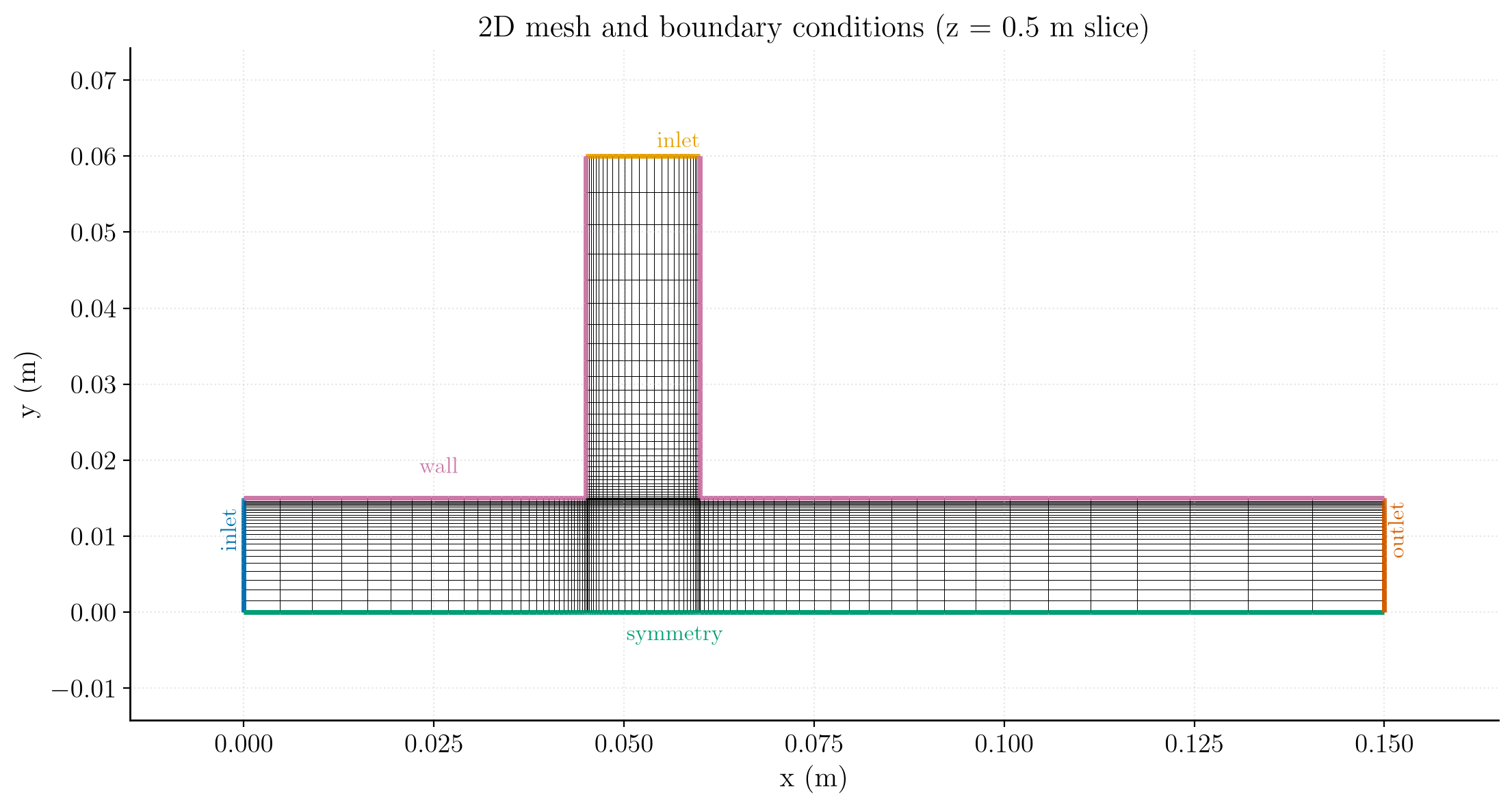
Figure 1: Mesh and boundary conditions (z = 0.5 m slice): inlets (blue/yellow),
outlet (orange), symmetry axis (green) and no-slip walls (pink).
The computational mesh is fully structured, composed of 3364 quadrilaterals (3510 points), refined toward the walls.
Numerical setup
| Setting | Value | Rationale |
|---|---|---|
| Velocity-pressure coupling | SIMPLEC | Robust segregated coupling for steady incompressible flow |
| Time-stepping | Local (pseudo) time step | Accelerates convergence to steady state by using a per-cell time step |
| Reference time step | \(\Delta t_\mathrm{ref}=0.1\ \mathrm{s}\) | Seed value, bounded by min/max factors \([0.1,\,1000]\) |
| Iterations | 200 | Steady state reached well within this budget |
| Initialization | \(\mathbf{u}=(1,0,0)\ \mathrm{m\,s^{-1}}\), \(Y_A = Y_B = 0\) | Uniform seed field |
| Convection scheme | 1st-order upwind | Accuracy for the flow; robustness and boundedness for the scalars |
| Species bounds | \(Y_i \in [0, 1]\) | Physical clipping of the mass fractions |
| Gradient reconstruction | Automatic | Default choice |
Three monitoring probes track convergence in the downstream channel at (\(x=0.06\), \(y=0.012\)), (\(x=0.08\), \(y=0.012\)) and (\(x=0.12\), \(y=0.012\)) m. They are sensitive indicators of when the mixing layer has reached steady state.
Running the simulation
The commands below start from the tutorial directory:
cd Inc_Species_Transport/
Option A: Graphical interface
code_saturne gui CASE/DATA/setup.xml &
The GUI opens the pre-configured setup.xml. Review the setup if you wish,
then launch the run with the gear (Run) button in the toolbar. To run in
parallel, set the number of processes under
Calculation management > Performance settings before launching.
Option B: Command line
The command-line launcher is run from inside the case directory:
cd CASE

# serial
code_saturne run

# parallel (e.g. 2 MPI ranks)
code_saturne run --n 2
With only 3364 cells this case runs comfortably in serial.
Each run creates a time-stamped directory CASE/RESU/<YYYYMMDD-HHMM>/ containing:
run_solver.log: solver log and residual history,monitoring/: probe time series (probes_*.csv),postprocessing/: volume and boundary fields in EnSight Gold format.
Results and verification
In the figures below the domain is mirrored across the symmetry axis (\(y=0\)) to display the full physical duct.
Velocity field
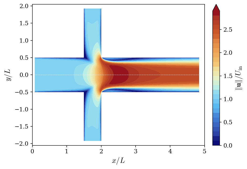
Figure 2: Nondimensional velocity magnitude $\|\mathbf{u}\|/U_\mathrm{in}$, with axes normalized by $L = 0.03$ m. The domain is mirrored across the symmetry axis (dashed line).
The vertical stream impinges on the horizontal one at the junction and the merged flow accelerates along the axis, leaving low-velocity regions behind the junction corners. Downstream, the flow relaxes toward a duct flow whose bulk velocity is set by mass conservation: both inlets have the same area and velocity, so the outlet bulk velocity is \(2 U_{in}\), i.e. \(\|\mathbf{u}\|/U_\mathrm{in} = 2\).
Species mass fractions
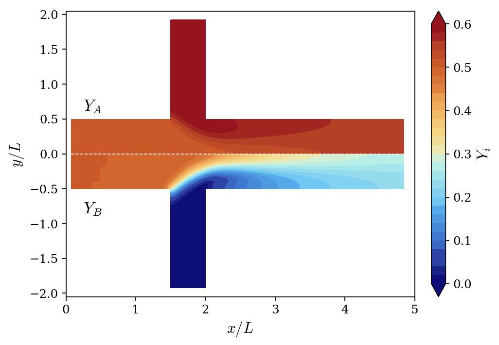
Figure 3: Mass fraction fields, with axes normalized by $L = 0.03$ m: $Y_A$ on the top half and $Y_B$ on the bottom (mirrored) half of the symmetry axis (dashed line). Both species share the same color scale.
Each inlet carries its own composition (\(Y_A = 0.5\) on the east stream, \(0.6\) on the north stream); the two streams mix in the junction region and the fields homogenize downstream, helped by the low Schmidt number.
Summary
This tutorial set up a steady, incompressible, turbulent mixing-channel simulation with passive species transport in code_saturne, using the k-\(\omega\) SST model and the N-1 equations closure for a three-species mixture. This case is a good baseline for RANS simulations involving species transport, before moving to composition-dependent properties or reacting flows.
References
Authors
Simvia - Questions, remarks and requests are welcome.