Packed Bed in a Duct

Browse this case on GitHub

A step-by-step tutorial for modelling a real porous medium in code_saturne, by combining the two features introduced separately in Inc_Head_Loss_Zone and Inc_Porous_Plug: a porosity zone for the kinematics (the flow accelerates in the reduced section) and a head-loss zone for the distributed friction of the solid matrix, with the coefficient calibrated from the Ergun correlation for a bed of spheres. This is the standard industrial recipe for packed beds, filters and tube bundles. The whole setup is done in the GUI: no mesh file, no user routine.

Maintained by Simvia, part of the tutoriel-code_saturne collection.

Learning objectives

After completing this tutorial you will be able to:

1. Give a single volume zone both natures (porosity and head losses).
2. Calibrate the head-loss coefficient from the Ergun correlation, taking care of the velocity convention (the resolved velocity is interstitial).
3. Choose a time step compatible with the stiffness of the head-loss term.

Prerequisites

Requirement	Detail
code_saturne	v9.1
Cases	Inc_Head_Loss_Zone and Inc_Porous_Plug (the two halves assembled here)

If code_saturne is not yet installed, build it from the official homepage, pull a ready-to-use Singularity image from the Open Simulation Center, or pull the Simvia Docker image before continuing.

Case files

Inc_Packed_Bed/
├── CASE/
│   └── DATA/
│       └── setup.xml            # pre-configured GUI case
├── FIGURES/                     # figures used in this README
└── README.md

There is no MESH directory (built-in cartesian mesher) and no SRC directory: everything is set in the GUI.

Physical model

The bed is a 0.2 m thick pack of \(d = 1\) mm spheres with porosity \(\varepsilon = 0.5\), crossed by air at the superficial velocity \(U = 1\ \mathrm{m\,s^{-1}}\). The Ergun correlation gives its pressure gradient as a viscous (Darcy) plus an inertial (Forchheimer) contribution:

\[ \frac{\Delta p}{L} = 150\,\frac{\mu (1-\varepsilon)^2}{\varepsilon^3 d^2}\, U + 1.75\,\frac{(1-\varepsilon)}{\varepsilon^3 d}\, \rho U^2 = 5400 + 8400 = 13800\ \mathrm{Pa\,m^{-1}} \]

i.e. \(\Delta p = 2760\) Pa across the bed: three orders of magnitude above the singular entry/exit effects seen in Inc_Porous_Plug, which is why a porosity zone alone badly under-predicts the resistance of a real bed.

Calibrating the head-loss coefficient

The head-loss source of code_saturne is \(-\frac{1}{2}\rho K |\mathbf{u}| \mathbf{u}\) per unit fluid volume, with \(\mathbf{u}\) the resolved velocity, which in a porosity zone is the interstitial one (\(u = U/\varepsilon = 2\ \mathrm{m\,s^{-1}}\) here). Matching the Ergun pressure drop at the operating point therefore gives

\[ K = \frac{\Delta p_{\mathrm{Ergun}}}{\frac{1}{2} \rho\, u^2 L} = \frac{2760}{0.5 \times 1.2 \times 2^2 \times 0.2} = 5750\ \mathrm{m^{-1}} \]

Two honest remarks on this calibration. First, it is a point calibration: the GUI head loss is quadratic in velocity, so the linear (Darcy) part of Ergun is folded into \(K\) at the nominal flow rate, and the case would not follow Ergun at other flow rates (a true Darcy-Forchheimer law needs the cs_user_head_losses user routine, where \(K\) can depend on \(|\mathbf{u}|\)). Second, mind the velocity convention: calibrating \(K\) with the superficial velocity instead of the interstitial one would miss the pressure drop by a factor \(1/\varepsilon^2 = 4\).

Flow parameters

Quantity	Symbol	Value	Source in setup.xml
Fluid (air-like)	\(\rho\), \(\mu\)	\(1.2\ \mathrm{kg\,m^{-3}}\), \(1.8 \times 10^{-5}\ \mathrm{Pa\,s}\)	density, molecular_viscosity
Superficial velocity	\(U\)	\(1\ \mathrm{m\,s^{-1}}\)	inlet/velocity_pressure/norm
Bed porosity, particle size	\(\varepsilon\), \(d\)	\(0.5\), \(1\) mm	porosities (MEG formula), Ergun inputs
Head-loss coefficient	\(K\)	\(5750\ \mathrm{m^{-1}}\) (isotropic)	head_losses/head_loss
Bed thickness	\(L\)	\(0.2\) m (\(x = 0.4\) to \(0.6\))	zone selector
Ergun pressure drop	\(\Delta p\)	\(2760\) Pa (\(13800\ \mathrm{Pa\,m^{-1}}\))	derived
Domain, mesh		\(1 \times 0.1 \times 0.02\) m, \(200 \times 20 \times 1\) cells	mesh_cartesian
Time	\(\Delta t\), \(N\)	\(2 \times 10^{-4}\) s, \(5000\) steps	time_parameters

Geometry and boundary conditions

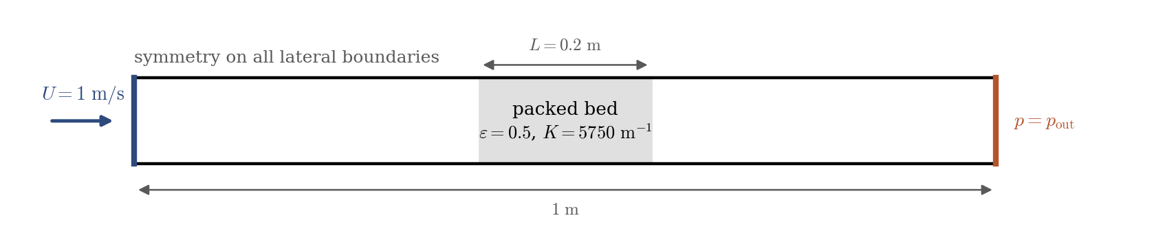
Figure 1: computational domain, identical to the two previous cases of the series; the middle zone now carries both natures.

Boundary	Location	Nature	Zone selector
Inlet	\(x = 0\)	Velocity inlet, \(1\ \mathrm{m\,s^{-1}}\)	X0
Outlet	\(x = 1\)	Free outlet	X1
SymY, SymZ	lateral faces	Symmetry	Y0 or Y1, Z0 or Z1

The packed-bed zone in the GUI

In Volume zones, the packed_bed zone (criterion box[0.4, -0.01, -0.01, 0.6, 0.11, 0.03]) gets both natures ticked: Porosity and Head losses. Then, in Volume conditions:

1. Porosity: isotropic model, MEG formula porosity = 0.5;
2. Head losses: \(K_{xx} = K_{yy} = K_{zz} = 5750\) (isotropic bed), identity transformation matrix.

Numerical setup

Setting	Value	Rationale
Velocity-pressure coupling	SIMPLEC	Standard segregated coupling
Velocity convection scheme	1st-order upwind (blending_factor 0)	Same rationale as Inc_Porous_Plug
Time-stepping	Fixed \(\Delta t = 2 \times 10^{-4}\) s, \(5000\) steps	Matched to the head-loss stiffness: \(K u \Delta t / 2 \approx 1\) (see below)
Turbulence	none (laminar)	Plug flow with slip boundaries
Initialization	\(u = U\) everywhere	Short transient
Probes	6 along the axis	2 upstream, 2 inside the bed, 2 downstream

A sizing lesson learned while building the case: the head-loss term introduces its own time scale, \(\tau_K = 2/(K u) \approx 1.7 \times 10^{-4}\) s here, far shorter than the convective one. With the time step of the previous episodes (\(2 \times 10^{-3}\) s, i.e. \(K u \Delta t/2 \approx 11\)), the coupled velocity-pressure iteration develops a slowly growing oscillation at the bed interfaces. Keeping \(K u \Delta t / 2 \lesssim 1\) restores a clean machine-level convergence: it is the head-loss analogue of the CFL condition.

Running the simulation

The commands below start from the tutorial directory:

cd Inc_Packed_Bed/

Option A: Graphical interface

code_saturne gui CASE/DATA/setup.xml &

The GUI opens the pre-configured setup.xml. Review the setup if you wish, then launch the run with the gear (Run) button in the toolbar.

Option B: Command line

The command-line launcher is run from inside the case directory:

cd CASE

# serial (a few seconds)
code_saturne run

Results

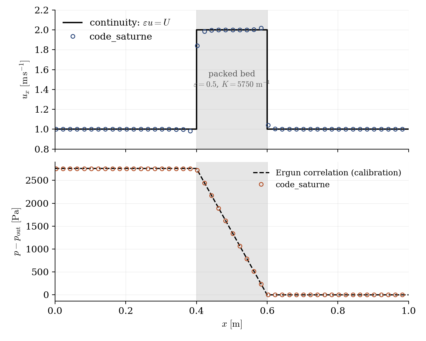
Figure 2: velocity (top) and pressure (bottom) along the duct at steady state. The interstitial velocity doubles in the bed exactly as in the porosity-only case; the pressure now falls linearly across it, with the slope of the Ergun calibration (dashed line).

The three signatures of the series come together:

• the velocity step is that of the porosity (\(u = U/\varepsilon = 2.000\ \mathrm{m\,s^{-1}}\), exact);
• the in-bed pressure gradient is \(-13800.0\ \mathrm{Pa\,m^{-1}}\), the calibrated Ergun slope to machine accuracy (the head-loss source is exactly the discretized formula), where the porosity-only case showed a flat plateau;
• the net pressure drop is \(2752\) Pa for \(2760\) Pa calibrated: the \(0.3\%\) difference is the residual entry/exit singular effects, now drowned by the matrix friction, as a real bed demands.

Summary

This tutorial assembled the porous-media recipe of code_saturne: one volume zone carrying both a porosity (kinematics: interstitial acceleration) and a head loss (distributed matrix friction), the latter calibrated from the Ergun correlation with the interstitial-velocity convention. The computed bed reproduces the calibrated gradient exactly and the end effects become negligible, closing the three-episode series started with Inc_Head_Loss_Zone and Inc_Porous_Plug.

References

• S. Ergun. Fluid flow through packed columns, Chem. Eng. Prog., 48:89-94, 1952.
• I.E. Idelchik. Handbook of Hydraulic Resistance, 4th edition, Begell House, 2007.
• code_saturne documentation

Authors

Simvia - Questions, remarks and requests are welcome.