Groundwater Flow and Tracer Transport in a Saturated Soil (Darcy, CDO)

Browse this case on GitHub

A step-by-step tutorial for the groundwater flow (GWF) module of code_saturne: saturated Darcy flow in a soil block, with a passive tracer advected by the seepage and spread by mechanical dispersion. The showcased feature is the CDO-based groundwater solver (cs_gwf_*): instead of the Navier-Stokes momentum equation, it solves the elliptic Richards equation for the hydraulic head, derives the Darcy flux, and transports a tracer on top of it. The case is validated against two exact references: Darcy's law (linear head, constant flux) and the Ogata-Banks advection-dispersion solution.

Maintained by Simvia, part of the tutoriel-code_saturne collection.

Learning objectives

After completing this tutorial you will be able to:

1. Activate the CDO groundwater flow module (cs_gwf_activate) for a saturated single-phase problem.
2. Define a soil (isotropic permeability, porosity) and a tracer equation (dispersivity, sorption) entirely from cs_user_parameters.cpp.
3. Impose hydraulic-head boundary conditions on the Richards equation and drive a Darcy flux through the domain.
4. Validate the head field against Darcy's law and the tracer front against the Ogata-Banks analytic solution.

Prerequisites

Requirement	Detail
code_saturne	v9.1 (built with the CDO module, default)
Tutorials	Inc_Species_Transport (scalar transport), Inc_Porous_Plug (porous media, for contrast)

If code_saturne is not yet installed, build it from the official homepage, pull a ready-to-use Singularity image from the Open Simulation Center, or pull the Simvia Docker image before continuing.

Case files

Gwf_Darcy_Tracer/
├── CASE/
│   ├── DATA/setup.xml               # mesh, time stepping, output only
│   └── SRC/
│       ├── cs_user_zones.cpp        # volume + inlet/outlet boundary zones
│       └── cs_user_parameters.cpp   # GWF model, soil, tracer, BCs, IC
├── FIGURES/
└── README.md

No mesh file: the 2D soil block is built by the built-in cartesian mesher.

Why is everything in C, not the GUI? In code_saturne v9.1 the groundwater module is driven by the CDO framework, activated in cs_user_model() with cs_gwf_activate(). The GUI's legacy groundwater panel is not wired to the v9.1 solver, so the model, soil, tracer and boundary conditions are all set in cs_user_parameters.cpp. The setup.xml only carries the mesh, the time stepping and the output.

Physical model

In a saturated porous medium, Darcy's law relates the seepage (Darcy) flux to the gradient of the hydraulic head \(h\):

\[\mathbf{q} = -K\,\nabla h,\]

where \(K\) is the hydraulic conductivity. Mass conservation of an incompressible fluid then gives the steady Richards equation (here a pure diffusion equation):

\[\nabla\!\cdot(K\,\nabla h) = 0.\]

The module solves this for \(h\), evaluates the Darcy flux \(\mathbf{q}\), and transports a passive tracer of normalized concentration \(C\):

\[\theta_s\,\frac{\partial C}{\partial t} + \nabla\!\cdot(\mathbf{q}\,C) - \nabla\!\cdot(\theta_s\,\mathbf{D}\,\nabla C) = 0,\]

with porosity \(\theta_s\) and a dispersion tensor built from the longitudinal and transverse dispersivities \(\alpha_L,\alpha_T\). The tracer therefore moves at the pore (interstitial) velocity \(v = q/\theta_s\) and spreads with \(D_L = \alpha_L\,v\).

Flow and transport parameters

Quantity	Symbol	Value
Domain	\(L \times H\)	\(100 \times 20\) m
Grid	\(n_x \times n_y\)	\(200 \times 20\) (2D)
Hydraulic conductivity	\(K\)	\(10^{-4}\) m/s
Porosity	\(\theta_s\)	\(0.4\)
Head difference	\(\Delta h\)	\(1\) m over \(L\)
Longitudinal dispersivity	\(\alpha_L\)	\(1\) m
Transverse dispersivity	\(\alpha_T\)	\(0.1\) m
Darcy flux	\(q = K\,\Delta h/L\)	\(10^{-6}\) m/s
Pore velocity	\(v = q/\theta_s\)	\(2.5\times10^{-6}\) m/s

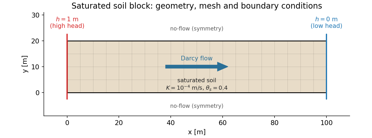
Figure 1: geometry, mesh and boundary conditions. A head difference between the left and right faces drives a left-to-right Darcy flow; top and bottom are no-flow.

Geometry and boundary conditions

The domain is a rectangular soil block. The two streamwise faces carry imposed hydraulic heads (Richards equation Dirichlet BCs): \(h = 1\) m at the inlet (left, group X0) and \(h = 0\) m at the outlet (right, group X1). The top and bottom faces are no-flow (CS_BOUNDARY_SYMMETRY, the CDO default). The tracer is injected at the inlet at \(C = 1\); the domain starts tracer-free (\(C = 0\)).

Numerical setup

Setting	Value	Rationale
Model	saturated, single phase (CS_GWF_MODEL_SATURATED_SINGLE_PHASE)	full saturation, no unsaturated zone
Discretization	CDO vertex-based	native framework of the v9.1 GWF module
Richards equation	steady	saturated flow with fixed head BCs
Tracer equation	unsteady	transient advection-dispersion
Time step	\(\Delta t = 10^{5}\) s	large steps allowed (implicit)
Duration	\(200\) steps (\(2\times10^{7}\) s)	tracer front reaches mid-domain

The Richards equation is solved once (it is steady); the Darcy flux is then constant in time and the tracer equation is advanced over the \(200\) steps.

Running the simulation

cd CASE
code_saturne run --n 4

The mesh is generated internally. The run writes CASE/RESU/<id>/ with the hydraulic head, the tracer concentration C and the Darcy flux field in postprocessing/, plus the Darcy flux balance across the boundary zones in run_solver.log.

Results and verification

Hydraulic head and Darcy flux. With a uniform conductivity the Richards equation has an exact linear solution \(h(x) = 1 - x/L\), and the Darcy flux is uniform. The solver reproduces both: the head is linear to machine precision, and the flux balance in the log reads \(q_x = 10^{-6}\) m/s (with \(q_y, q_z\) at numerical zero), matching \(q = K\,\Delta h/L = 10^{-4}\times(1/100)\) exactly.

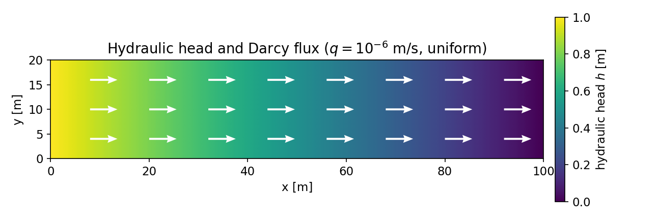
Figure 2: hydraulic head field and the uniform Darcy flux ($q = 10^{-6}$ m/s).

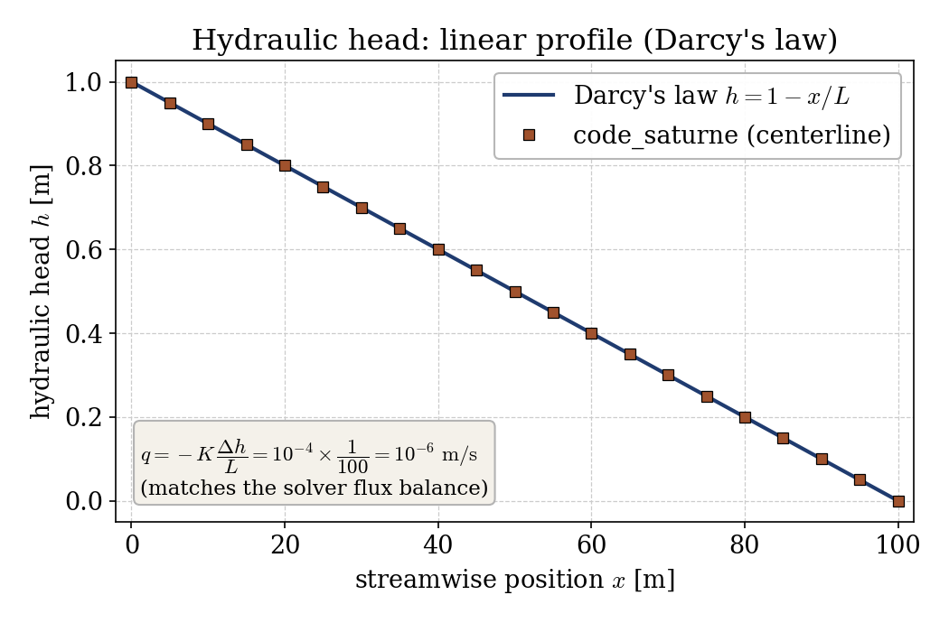
Figure 3: centerline head versus the analytic Darcy solution. The flux follows directly from the slope.

Tracer front. For continuous injection into a semi-infinite column with a uniform velocity, the advection-dispersion equation has the Ogata-Banks (1961) solution

\[\frac{C}{C_0} = \tfrac12\left[\operatorname{erfc}\!\frac{x - v t}{2\sqrt{D_L t}} + \exp\!\Big(\frac{v x}{D_L}\Big)\operatorname{erfc}\!\frac{x + v t}{2\sqrt{D_L t}}\right].\]

With \(v = q/\theta_s = 2.5\times10^{-6}\) m/s and \(D_L = \alpha_L v\), the computed front matches the analytic curve at every output time: the front advances at the pore velocity (\(x_{0.5}\approx v t\)) and broadens as \(\sqrt{D_L t}\).

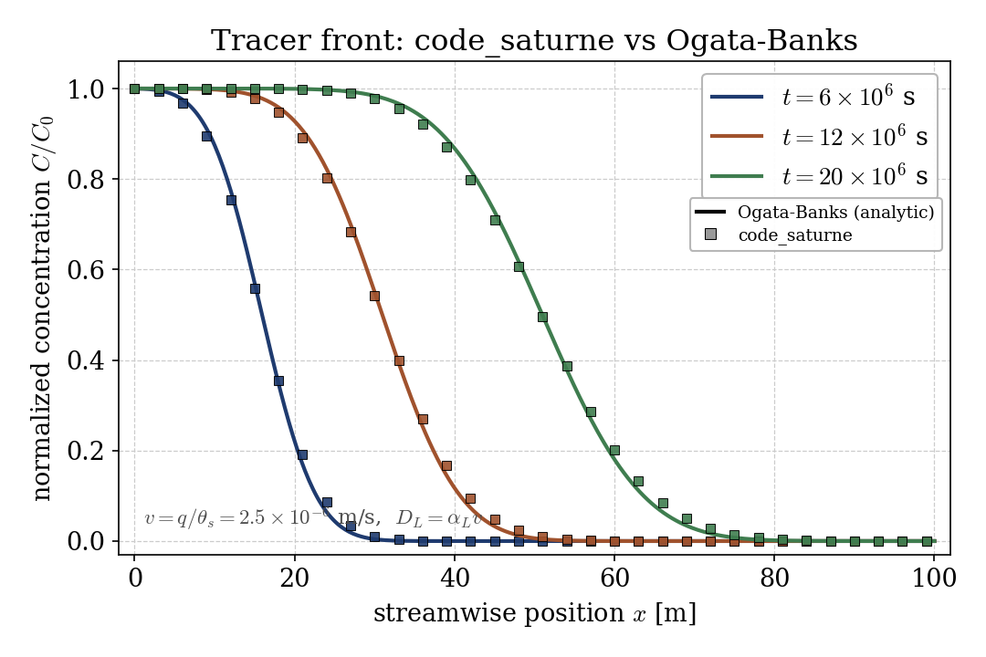
Figure 4: tracer front (symbols) versus the Ogata-Banks solution (lines) at three times. The pore velocity and the dispersive spreading are both recovered.

The agreement confirms the whole chain: the head solve, the derived Darcy flux, and the dispersive transport on top of it. The only visible departure is a sub-percent lead of the numerical front at the latest time, the expected effect of the finite (semi-infinite in the analytic model) column length.

Summary

This tutorial solved a saturated groundwater flow with the CDO groundwater module: the Richards equation fixed a linear hydraulic head and a uniform Darcy flux (\(q = K\,\Delta h/L\)), and a passive tracer injected at the inlet was advected and dispersed on top of it. Both the head (Darcy's law) and the tracer front (Ogata-Banks) match their exact references. The lesson that carries beyond this case: in code_saturne the groundwater module replaces the momentum equation with Darcy's law and is set up through the CDO API in cs_user_parameters.cpp, a different workflow from the finite-volume Navier-Stokes cases.

References

• A. Ogata, R. B. Banks. A solution of the differential equation of longitudinal dispersion in porous media, U.S. Geological Survey Professional Paper 411-A, 1961.
• J. Bear. Dynamics of Fluids in Porous Media, Elsevier, 1972.
• code_saturne documentation

Authors

Simvia. Questions, remarks and requests are welcome.