The Ekman Layer: Wind Veering under Coriolis (atmo)

Browse this case on GitHub

A step-by-step tutorial for the Coriolis effect in an atmospheric boundary layer with code_saturne: the Ekman layer. Away from the ground the wind is in geostrophic balance (pressure gradient against Coriolis) and blows along the isobars; near the rough ground friction slows it and it veers (turns direction) with height, tracing the classic Ekman spiral. The showcased feature is the Coriolis source term (omega) combined with a geostrophic forcing.

Maintained by Simvia, part of the tutoriel-code_saturne collection.

Learning objectives

After completing this tutorial you will be able to:

1. Activate the Coriolis source term via the rotation vector (\(\omega_z = f/2\)).
2. Impose a geostrophic wind through a constant body force in geostrophic balance with the Coriolis force.
3. Set up a horizontally homogeneous 1D column (periodic in both horizontal directions) over a rough ground.
4. Read the Ekman spiral on a hodograph and the surface veering angle.

Prerequisites

Requirement	Detail
code_saturne	v9.1
Tutorials	Atmo_Neutral_BoundaryLayer (neutral surface layer, rough wall)

If code_saturne is not yet installed, build it from the official homepage, pull a ready-to-use Singularity image from the Open Simulation Center, or pull the Simvia Docker image before continuing.

Case files

Atmo_Ekman_Layer/
├── CASE/
│   ├── DATA/setup.xml                    # neutral atmo, Coriolis (omega_z), k-epsilon
│   └── SRC/
│       ├── cs_user_source_terms.cpp      # geostrophic body force
│       └── cs_user_initialization.cpp    # start from the geostrophic wind
├── FIGURES/
└── README.md

No mesh file: the vertical column is built by the built-in cartesian mesher.

Physical model

In the free atmosphere, steady and frictionless, the horizontal momentum balance is geostrophic: the pressure-gradient force balances the Coriolis force,

\[f\,\mathbf{\hat z}\times\mathbf{U}_g = -\tfrac1\rho\nabla p,\]

with \(f = 2\Omega\sin\varphi\) the Coriolis parameter (\(\varphi\) the latitude). The result is the geostrophic wind \(\mathbf{U}_g\), blowing along the isobars.

Near the ground, friction removes momentum and breaks this balance: the wind slows and turns toward low pressure. The three-way balance (pressure gradient, Coriolis, friction) gives a wind that rotates with height, the Ekman spiral, from a reduced, veered wind at the surface to the full geostrophic wind aloft.

Here the Coriolis force is set through the rotation vector \(\omega_z = f/2\), and the geostrophic pressure gradient is imposed as a constant body force \((0,\rho f G,0)\), which in geostrophic balance yields \(\mathbf{U}_g = (G,0,0)\). The column is periodic in both horizontal directions (the flow varies only with height) over a rough ground.

Flow parameters

Quantity	Symbol	Value
Latitude	\(\varphi\)	\(45\)°
Coriolis parameter	\(f = 2\Omega\sin\varphi\)	\(1.03\times10^{-4}\) s⁻¹
Geostrophic wind	\(G\)	\(10\) m/s
Roughness length	\(z_0\)	\(0.1\) m
Domain height	\(H\)	\(5000\) m
Turbulence		\(k\)-\(\varepsilon\)

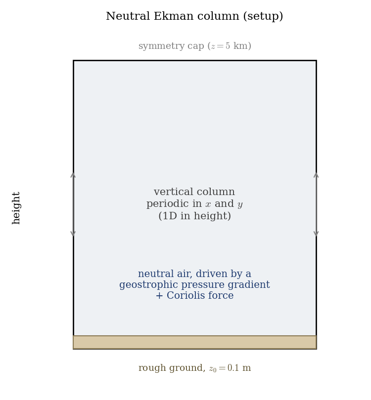
Figure 1: the setup. A tall vertical column, periodic in the horizontal (so the flow varies only with height), over a rough ground, driven by a geostrophic pressure gradient with the Coriolis force.

Geometry and boundary conditions

A vertical column, \(z\) the vertical, periodic in \(x\) and \(y\) (horizontally homogeneous). The ground (Z0) is a rough wall (\(z_0 = 0.1\) m) and the top (Z1) is a symmetry plane. The Coriolis rotation and the geostrophic body force act throughout the volume.

Numerical setup

Neutral atmospheric model, \(k\)-\(\varepsilon\) turbulence, constant density. The Coriolis term is set with \(\omega_z = f/2\); cs_user_source_terms.cpp applies the geostrophic force. The run is advanced well past one inertial period (\(2\pi/f \approx 17\) h) so the inertial oscillation is damped and the profile is steady.

Running the simulation

cd CASE
code_saturne run --n 4

The mesh is generated internally. The run writes CASE/RESU/<id>/ with the velocity and turbulence fields.

Results and verification

The wind rotates with height, the signature of the Ekman layer. The profiles are shown normalized: the wind by the geostrophic speed \(G\) and the height by the Ekman depth \(\delta = \sqrt{2\,\nu_t/f}\) (here \(\delta \approx 1.5\) km from the turbulent eddy viscosity), which makes the spiral universal. On the hodograph (\(v/G\) against \(u/G\)), the wind starts at the ground with a reduced, veered vector, rises, slightly overshoots the geostrophic value (\(u/G > 1\)) and then curls back toward the geostrophic point \(u/G = 1\), \(v/G = 0\) aloft, the start of the Ekman coil.

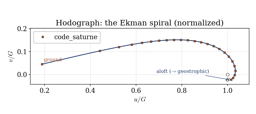
Figure 2: hodograph (the Ekman spiral), normalized by $G$. The wind vector turns and grows from the ground, overshoots $G$ and curls back toward it aloft.

The components make the same point: the along-wind \(u/G\) rises from a small surface value to about \(1\) aloft, while the cross-wind \(v/G\) is largest near the ground and vanishes aloft. The surface wind is veered about \(12\)° from the geostrophic direction.

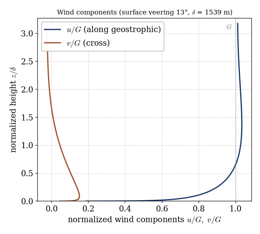
Figure 3: normalized wind components $u/G,\ v/G$ versus $z/\delta$. The along-wind tends to $G$ aloft; the cross-wind marks the veering, concentrated near the ground.

The classic laminar Ekman solution (constant eddy viscosity) predicts a \(45\)° surface veering; a turbulent boundary layer with a height-dependent eddy viscosity veers much less, typically \(10\)-\(30\)°, and the \(\approx 12\)° found here is in that range. The point of the case is the veering with height produced by the Coriolis force, not a match to the constant-viscosity spiral.

Summary

This tutorial added the Coriolis force to a neutral atmospheric column and drove it with a geostrophic body force. The wind reaches the geostrophic value aloft and veers toward the ground, tracing the Ekman spiral, with a surface veering of about \(12\)° for this turbulent boundary layer. The lesson that carries beyond this case: the Coriolis source term (set through the rotation vector) turns a plain boundary layer into a rotating-frame atmospheric one, the mechanism behind the wind turning with height in the real atmosphere.

References

• V. W. Ekman. On the influence of the Earth's rotation on ocean currents, Arkiv för Matematik, Astronomi och Fysik 2, 1-53, 1905.
• J. R. Garratt. The Atmospheric Boundary Layer, Cambridge University Press, 1992.
• code_saturne documentation

Authors

Simvia. Questions, remarks and requests are welcome.