Turbulent Channel Flow (Periodic, Law of the Wall)¶

Browse this case on GitHub

A step-by-step tutorial for a fully-developed turbulent channel in code_saturne: an incompressible RANS flow between two parallel walls, made streamwise-periodic and driven by a constant momentum source term instead of an inlet/outlet. The tutorial's purpose is that periodic + source-term workflow and its canonical validation: a wall-resolved computation that recovers the law of the wall ($u^+$ versus $y^+$) at $Re_\tau = 395$.

Maintained by Simvia, part of the tutoriel-code_saturne collection.

Learning objectives¶

After completing this tutorial you will be able to:

Build a streamwise-periodic channel with the built-in cartesian mesher, using a parabolic grading to resolve both walls ($y^+ \approx 1$).
Drive a periodic flow with a constant momentum source term (cs_user_source_terms) that replaces the mean pressure gradient and fixes the friction Reynolds number by construction.
Run a wall-resolved k-$\omega$ SST RANS computation to steady state.

Prerequisites¶

Requirement	Detail
code_saturne	v9.1
Tutorials	Inc_Streamwise_Periodic (periodicity + source term), Inc_Turbulent_Plate (RANS near walls)

If code_saturne is not yet installed, build it from the official homepage, pull a ready-to-use Singularity image from the Open Simulation Center, or pull the Simvia Docker image before continuing.

Case files¶

Inc_Turbulent_Channel/
├── CASE/
│   ├── DATA/setup.xml                # cartesian mesh, periodicity, k-omega SST
│   └── SRC/cs_user_source_terms.cpp  # constant streamwise body force f_x
├── FIGURES/                          # figures used in this README
└── README.md

No mesh file: the domain is built by the built-in cartesian mesher from setup.xml, so the case is fully self-contained.

Physical model¶

The flow is incompressible, statistically steady and fully turbulent between two parallel walls a distance $2h$ apart. It is closed with the k-$\omega$ SST model, integrated down to the wall (no wall function needed), so the profile is resolved through the viscous sublayer.

Because the channel is periodic in the streamwise direction there is no inlet or outlet, and the mean pressure gradient that would drive the flow is instead supplied as a constant body force $f_x$ added to the streamwise momentum equation. At statistical steady state this force is balanced exactly by the wall friction, which pins the wall shear and therefore the friction velocity:

\[ f_x = \frac{\rho\,u_\tau^2}{h} \quad\Longrightarrow\quad \tau_w = f_x\,h = \rho\,u_\tau^2 . \]

The case is written in wall units: $h = 1$, $\rho = 1$, $u_\tau = 1$, so $f_x = 1$ and the molecular viscosity alone sets the friction Reynolds number, $Re_\tau = u_\tau h/\nu = 1/\nu$. Choosing $\nu = 1/395$ gives $Re_\tau = 395$. The bulk velocity is then an output of the run.

The near-wall mean profile follows the law of the wall:

\[ u^+ = y^+ \ (\text{viscous sublayer}, y^+ \lesssim 5), \qquad u^+ = \tfrac{1}{\kappa}\ln y^+ + B \ (\text{log region}, y^+ \gtrsim 30), \]

with $\kappa = 0.41$, $B = 5.2$, and $u^+ = U_x/u_\tau$, $y^+ = y_w u_\tau/\nu$ ($y_w$ the distance to the nearest wall).

Flow parameters (wall units)¶

Quantity	Symbol	Value	Source in `setup.xml`
Half-height	$h$	$1$	mesh
Density	$\rho$	$1$	`fluid_properties/density`
Friction velocity	$u_\tau$	$1$ (by construction)	momentum balance
Molecular viscosity	$\nu$	$1/395 \approx 2.532\times10^{-3}$	`molecular_viscosity`
Streamwise body force	$f_x = \rho u_\tau^2/h$	$1$	`cs_user_source_terms.cpp`
Friction Reynolds number	$Re_\tau = u_\tau h/\nu$	$395$	derived

To run a different $Re_\tau$, change a single number: $\nu = 1/Re_\tau$.

Geometry and boundary conditions¶

The domain is a cartesian box, $2h$ long in $x$, $2h$ tall in $y$ (wall to wall), and one cell thick in $z$. The wall-normal direction uses a parabolic grading that refines toward both walls (first cell centre at $y^+ \approx 0.4$). Because the mean flow is statistically one-dimensional, the streamwise and spanwise extents can be small.

Boundary	Group	Nature	Prescribed
bottom, top	`Y0`, `Y1`	no-slip wall	$\mathbf{u} = 0$
inlet/outlet planes	`X0`, `X1`	periodic (translation)	streamwise periodicity
spanwise planes	`Z0`, `Z1`	symmetry	quasi-2D

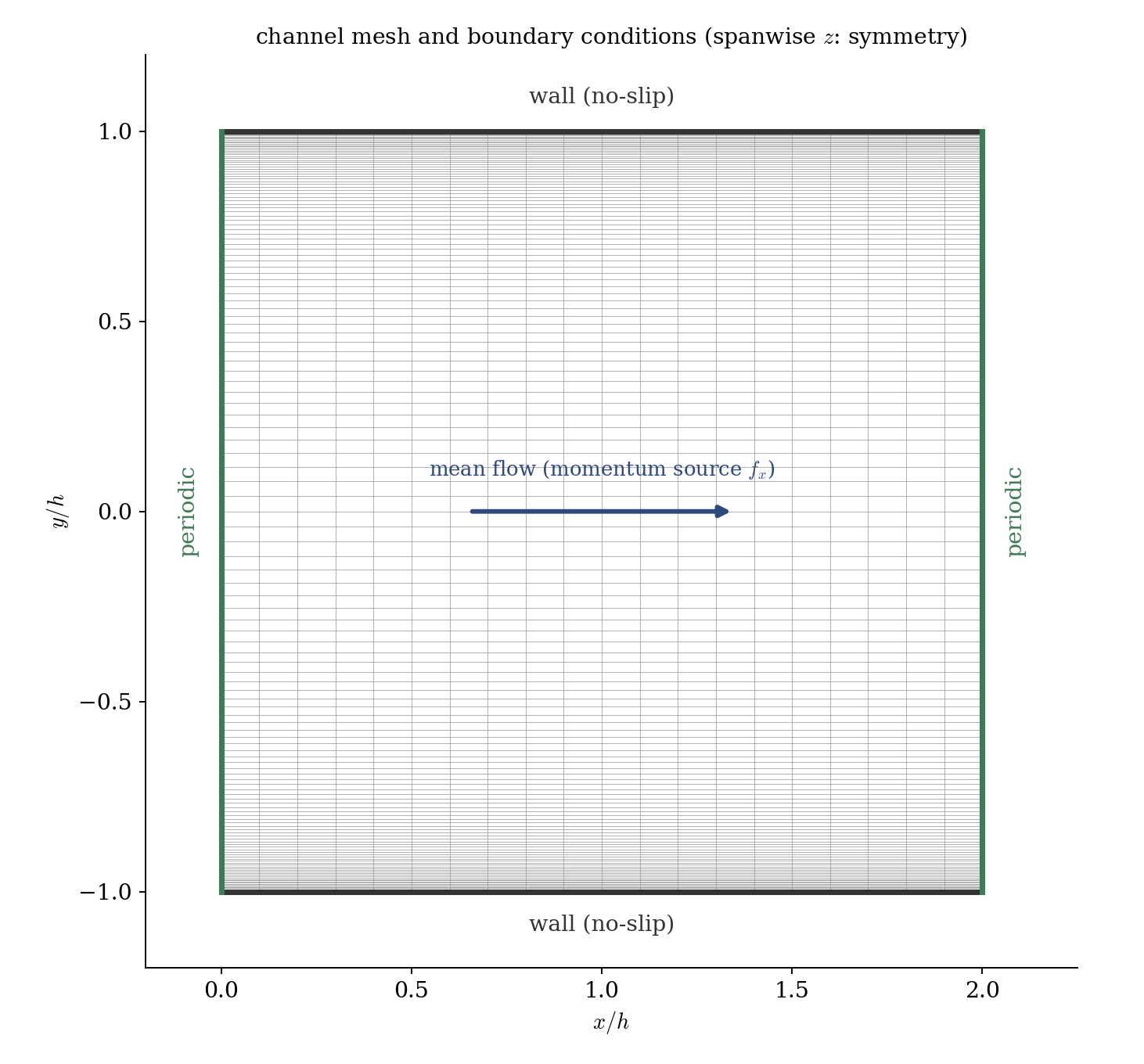
Cartesian channel mesh graded toward both walls, with no-slip walls top and bottom, streamwise periodicity left and right, spanwise symmetry, and the streamwise momentum source arrow.
Figure 1: the cartesian mesh (coordinates in half-heights $h$) and boundary conditions. The wall-normal grading (parabolic) clusters cells at both no-slip walls; the streamwise planes are periodic and the flow is driven by the constant momentum source $f_x$; the spanwise planes are symmetry.

Numerical setup¶

Setting	Value	Rationale
Coupling	SIMPLEC	robust segregated incompressible coupling
Convection scheme	2nd-order centred	low numerical diffusion
Time-stepping	local (pseudo) time step	drives to steady state
Turbulence	k-$\omega$ SST, wall-resolved ($y^+ \approx 0.4$)	resolves the sublayer, no wall function
Driving	constant momentum source $f_x = 1$	replaces the mean pressure gradient
Iterations	to residual plateau (a few thousand)	steady state

The momentum source is added in cs_user_source_terms.cpp as an explicit term $f_x$ integrated over each cell volume, on the streamwise velocity component only.

Running the simulation¶

The commands below start from the tutorial directory.

Graphical interface¶

code_saturne gui CASE/DATA/setup.xml &

Command line¶

cd CASE
code_saturne run                 # serial
code_saturne run --n 4      # parallel

The mesh is generated internally, so no mesh import is needed. Each run writes a timestamped CASE/RESU/<id>/ with run_solver.log, the monitoring probe and the EnSight fields in postprocessing/.

Results and verification¶

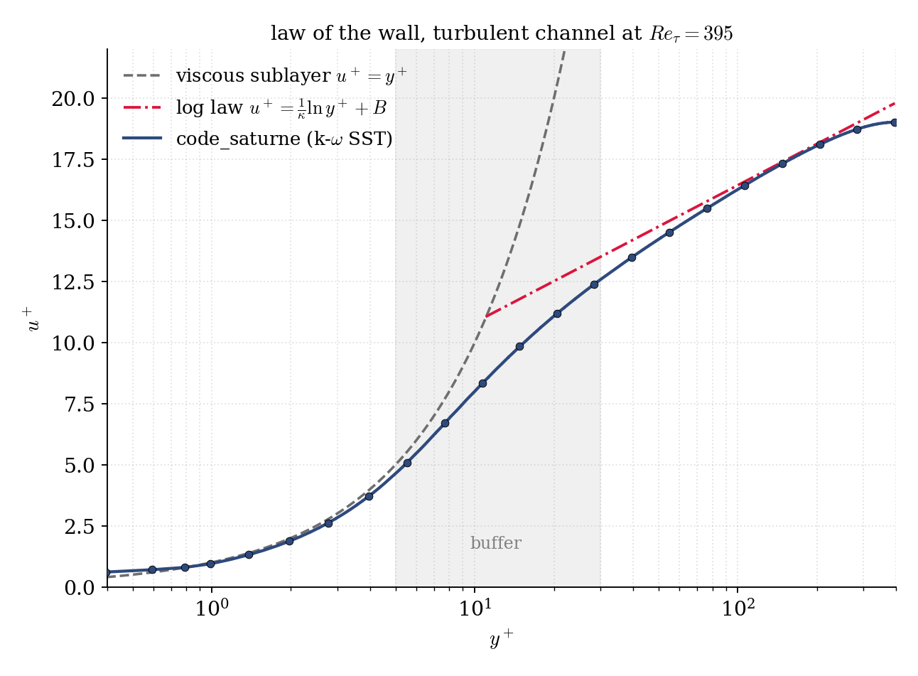
Computed u+ versus y+ following the viscous sublayer u+=y+, transitioning through the buffer layer, and matching the logarithmic law in the log region.
Figure 2: mean velocity in wall units, $u^+$ versus $y^+$. The wall-resolved k-$\omega$ SST follows $u^+ = y^+$ in the viscous sublayer, bends through the buffer layer, and lies on the logarithmic law $u^+ = \tfrac{1}{\kappa}\ln y^+ + B$ ($\kappa = 0.41$, $B = 5.2$) in the log region.

The validation is the law of the wall itself (Figure 2): the profile recovers $u^+ = y^+$ through the viscous sublayer and lies on the logarithmic law in the log region, where the match is close ($u^+ = 16.3$ at $y^+ = 100$ against $16.4$ from the log law, and $18.1$ against $18.1$ at $y^+ = 200$).

Summary¶

This tutorial built a fully-developed turbulent channel entirely from the built-in cartesian mesher, made it streamwise-periodic, and drove it with a constant momentum source term that fixes $Re_\tau = 395$ by construction. A wall-resolved k-$\omega$ SST computation recovers the law of the wall (viscous sublayer $u^+ = y^+$ and the logarithmic region). The lesson that carries beyond this case: a periodic domain plus a momentum source is the natural, boundary-condition-free way to compute a fully-developed internal flow.

References¶

R. D. Moser, J. Kim, N. N. Mansour. Direct numerical simulation of turbulent channel flow up to $Re_\tau = 590$, Physics of Fluids 11, 943-945, 1999.
code_saturne documentation

Authors¶

Simvia. Questions, remarks and requests are welcome.

Quantity	Symbol	Value	Source in `setup.xml`
Half-height	\(h\)	\(1\)	mesh
Density	\(\rho\)	\(1\)	`fluid_properties/density`
Friction velocity	\(u_\tau\)	\(1\) (by construction)	momentum balance
Molecular viscosity	\(\nu\)	\(1/395 \approx 2.532\times10^{-3}\)	`molecular_viscosity`
Streamwise body force	\(f_x = \rho u_\tau^2/h\)	\(1\)	`cs_user_source_terms.cpp`
Friction Reynolds number	\(Re_\tau = u_\tau h/\nu\)	\(395\)	derived