Humid Atmosphere: Cloud Formation from a Meteo Profile (atmo)¶

Browse this case on GitHub

A step-by-step tutorial for the humid atmosphere model of the atmospheric flows module (atmo) in code_saturne. Building on the meteo-file case, it switches on the humid model, which transports the total water and the liquid potential temperature and diagnoses condensation: where the air reaches saturation, cloud liquid water appears. The showcased feature is the humid model and its saturation adjustment, demonstrated on a moist meteo profile that forms a cloud layer aloft.

Maintained by Simvia, part of the tutoriel-code_saturne collection.

Learning objectives¶

After completing this tutorial you will be able to:

Activate the humid atmospheric model (total water, liquid potential temperature, cloud diagnostics).
Provide a humid meteo profile (a total-water column in the meteo file).
Understand the saturation adjustment: cloud liquid water forms where the total water exceeds the saturation value $q_{sat}(T,p)$.
Read the cloud fields (LiqWater, cloud fraction) and interpret the cloud layer.

Prerequisites¶

Requirement	Detail
code_saturne	v9.1
Tutorials	Atmo_Meteo_Profile (meteo-file workflow), Atmo_Neutral_BoundaryLayer

If code_saturne is not yet installed, build it from the official homepage, pull a ready-to-use Singularity image from the Open Simulation Center, or pull the Simvia Docker image before continuing.

Case files¶

Atmo_Humid_Cloud/
├── CASE/
│   ├── DATA/
│   │   ├── setup.xml                     # humid atmo model, read_meteo_data on, k-epsilon
│   │   └── meteo                         # humid profile (temperature + total water)
│   └── SRC/
│       ├── cs_user_zones.cpp             # boundary zones
│       ├── cs_user_boundary_conditions.cpp   # meteo inlet + rough wall (in C)
│       └── cs_user_initialization.cpp    # initial fields (incl. total water, droplets)
├── FIGURES/
└── README.md

No mesh file: the vertical slice is built by the built-in cartesian mesher. Boundary conditions are set in C for the same reason as the meteo-file case (the v9.1 GUI meteo-boundary path is not wired to the preprocessor).

Physical model¶

The humid atmospheric model carries two conserved quantities: the total water content $q_w$ (vapour plus condensed water) and the liquid potential temperature. Only $q_w$ is transported by the flow (advection and turbulent diffusion); the split between vapour and liquid is diagnosed at each point.

The saturation water content is a thermodynamic function of temperature and pressure, from a Clausius-Clapeyron (Magnus) law for the saturation vapour pressure $e_s(T)$:

\[e_s(T) = 611.2\,\exp\!\Big(\tfrac{17.62\,T_C}{243.12 + T_C}\Big),\qquad q_{sat} = \frac{0.622\,e_s}{p - 0.378\,e_s}.\]

The model then applies a saturation adjustment: the excess of total water above saturation condenses into cloud liquid water,

\[q_l = \max\!\big(0,\; q_w - q_{sat}\big),\]

and the vapour stays at $q_{sat}$. The condensation releases latent heat, which warms the air and raises $q_{sat}$, so the adjustment is an equilibrium rather than a plain subtraction: this coupling is exactly why the conserved thermal variable is the liquid potential temperature. The buoyancy accounts for the water loading and the hydrostatic pressure is solved.

Because $q_{sat}$ decreases with height (the air cools), a layer with enough moisture becomes saturated above a certain altitude (the cloud base), while it stays clear below. Here the meteo file prescribes a moist layer between about $250$ and $700$ m (relative humidity above $100\%$), unsaturated near the ground (no fog) and dry aloft, so a cloud layer forms in between.

Cloud droplet number. The meteo file also carries a droplet number concentration ($100\ \mathrm{cm^{-3}}$ here). It does not control whether the cloud forms: condensation is set purely by $q_w > q_{sat}$ (running with zero droplets gives the same liquid water). The droplet number only sets the mean droplet radius, $r \propto (q_l/N_c)^{1/3}$, used for the microphysics and the radiative properties of the cloud.

Setup parameters¶

Quantity	Value
Domain	$1000 \times 1000$ m (vertical slice)
Atmosphere	humid (dry, neutral base state, $T_{surf} = 15$°C)
Total water (moist layer)	$\approx 10.3$ g/kg (RH $> 100\%$)
Roughness length	$z_0 = 0.1$ m
Turbulence	$k$-$\varepsilon$

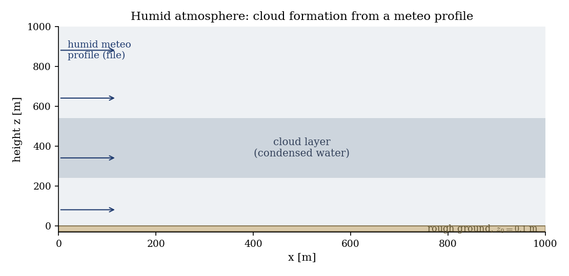
Vertical slice: a humid meteo profile enters from the west over a rough ground, and a cloud layer forms between about 250 and 540 m.
Figure 1: the humid meteo profile enters from the west; a cloud layer forms aloft where the air is saturated.

Geometry and boundary conditions¶

Vertical slice, $z$ the vertical. As in the meteo-file case, the west face and the top are meteo inlets (CS_INLET, filled from the profile), the east face is an outlet, the ground is a rough wall, and the spanwise sides are symmetry. The inlet total water follows the humid profile from the meteo file.

Numerical setup¶

Humid atmospheric model with read_meteo_data on. The velocity, turbulence, liquid potential temperature, total water and droplet number are initialized in cs_user_initialization.cpp; the meteo inlet then drives the profiles. The run advances to a steady state ($2000$ steps).

Running the simulation¶

cd CASE
code_saturne run --n 4

The mesh is generated internally and the meteo file is read at start-up. The run writes CASE/RESU/<id>/ with the velocity, total water (TotWater), cloud liquid water (LiqWater) and cloud fraction (Nebulo_frac).

Results¶

A cloud layer forms aloft: the liquid water is zero near the ground, rises to a maximum around $400$ m and vanishes again near $540$ m, exactly the band where the total water exceeds the saturation value.

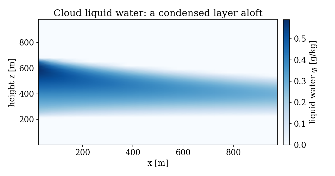
Two-dimensional field of cloud liquid water: a condensed band between about 250 and 540 m, thickest near the inlet and thinning downstream.
Figure 2: cloud liquid water field. The condensed layer thins downstream as turbulent mixing entrains drier air from above and below.

The mechanism is the saturation adjustment: plotting the total water and the saturation value against height, the cloud (shaded) sits exactly where $q_w > q_{sat}$, and the diagnosed liquid water $q_l$ peaks there, consistent with $q_l \approx q_w - q_{sat}$.

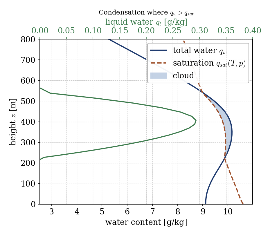
Vertical profiles of total water and saturation humidity; the cloud region is shaded where total water exceeds saturation, and the liquid water peaks there.
Figure 3: total water $q_w$ and saturation $q_{sat}(T,p)$ versus height. Cloud liquid water $q_l$ (green) appears where $q_w > q_{sat}$ (shaded).

This is a demonstration of the humid model rather than a validated case: the cloud thickness and liquid-water amount depend on the prescribed profile and on the turbulent mixing, which erodes the moist layer downstream (visible in Figure 2).

Summary¶

This tutorial switched on the humid atmospheric model and fed it a moist meteo profile: where the total water exceeds the saturation value, code_saturne condenses the excess into cloud liquid water, forming a cloud layer aloft. The lesson that carries beyond this case: the humid model adds the water cycle (vapour, condensation, cloud) to the atmospheric solver through the total water and the saturation adjustment, the entry point to fog, stratocumulus and cloudy boundary-layer studies.

References¶

J. R. Garratt. The Atmospheric Boundary Layer, Cambridge University Press, 1992.
R. B. Stull. An Introduction to Boundary Layer Meteorology, Kluwer, 1988.
code_saturne atmospheric flows documentation

Authors¶

Simvia. Questions, remarks and requests are welcome.

Quantity	Value
Domain	\(1000 \times 1000\) m (vertical slice)
Atmosphere	humid (dry, neutral base state, \(T_{surf} = 15\)°C)
Total water (moist layer)	\(\approx 10.3\) g/kg (RH \(> 100\%\))
Roughness length	\(z_0 = 0.1\) m
Turbulence	\(k\)-\(\varepsilon\)