2D Mixer Vessel (Frozen Rotor)

Browse this case on GitHub

A step-by-step tutorial for simulating a baffled stirred tank with the turbomachinery module of code_saturne: a four-blade impeller rotating at 1000 rpm inside a cylindrical vessel equipped with four baffles, computed with the frozen rotor approach. The case is a compact demonstration of the turbomachinery workflow: a rotor zone defined by a geometric criterion, blades and baffles created as thin walls, and monitoring probes to assess convergence.

Maintained by Simvia, part of the tutoriel-code_saturne collection.

Learning objectives

After completing this tutorial you will be able to:

1. Enable the frozen rotor turbomachinery model and define the rotor zone with a geometric criterion.
2. Create internal zero-thickness walls (thin walls) from geometric selectors, without meshing them.
3. Set up a RANS computation with the k-ε Linear Production model and scalable wall functions.
4. Place monitoring probes and use them to assess the convergence of a pseudo-steady run.

Prerequisites

Requirement	Detail
code_saturne	v9.1
Background	RANS turbulence modelling basics; a first incompressible tutorial such as Inc_Inviscid_Hydrofoil

If code_saturne is not yet installed, build it from the official homepage, pull a ready-to-use Singularity image from the Open Simulation Center, or pull the Simvia Docker image before continuing.

Case files

Tbm_Mixer_Vessel_2D/
├── CASE/
│   └── DATA/
│       └── setup.xml            # pre-configured GUI case
├── MESH/
│   └── mixerVessel2D.msh        # annular quasi-2D mesh (gmsh)
├── FIGURES/                     # figures used in this README
└── README.md

Note that the mesh contains neither the blades nor the baffles: it is a plain annulus. Both are inserted at run time as thin walls (see below).

Physical model

The flow is incompressible and turbulent. Its physics is governed by the impeller Reynolds number, built on the rotation rate \(N\) (in revolutions per second) and the impeller diameter \(D = 0.1\) m:

\[ Re = \frac{N D^2}{\nu} = \frac{16.67 \times 0.1^2}{10^{-5}} \approx 1.7 \times 10^4 \]

Turbulence is modelled with the k-ε Linear Production variant (which limits the spurious production of turbulent energy in highly strained regions, such as the blade tips) and scalable wall functions.

The frozen rotor approach computes a steady approximation of the rotor-stator interaction: the equations are solved in the rotating frame inside the rotor zone (with the corresponding Coriolis and centrifugal terms) and in the fixed frame outside, with the rotor frozen at one angular position. It is the cheapest turbomachinery model, and the natural first step before a transient rotor-stator computation with mesh rotation.

Flow parameters

Quantity	Symbol	Value	Source in setup.xml
Density	\(\rho\)	\(1\ \mathrm{kg\,m^{-3}}\)	density
Molecular viscosity	\(\mu\)	\(10^{-5}\ \mathrm{Pa\,s}\)	molecular_viscosity
Rotation rate	\(\omega\)	\(104.72\ \mathrm{rad\,s^{-1}}\) (1000 rpm)	turbomachinery/rotor/velocity
Blade tip speed	\(\omega\, r_{tip}\)	\(5.24\ \mathrm{m\,s^{-1}}\)	derived (\(r_{tip} = 0.05\) m)
Impeller Reynolds number	\(Re\)	\(1.7 \times 10^4\)	derived

Geometry and boundary conditions

The vessel is an annulus of outer radius \(0.1\) m (tank wall) and inner radius \(0.02\) m (hub), extruded one cell over a thickness of \(0.01\) m: the computation is quasi-2D. From the axis outwards:

Radius [m]	Element
\(0.02\)	hub (no-slip wall)
\(0.02 - 0.05\)	4 impeller blades at \(0°/90°/180°/270°\) (thin walls)
\(0.06\)	rotor/stator interface (rotor/criteria, dashed circle in Figure 3)
\(0.07 - 0.10\)	4 baffles at \(45°/135°/225°/315°\) (thin walls)
\(0.10\)	tank wall (no-slip wall)

The mesh (MESH/mixerVessel2D.msh) is a structured polar grid of \(96 \times 32 \times 1 = 3072\) hexahedra, radially refined towards the hub:

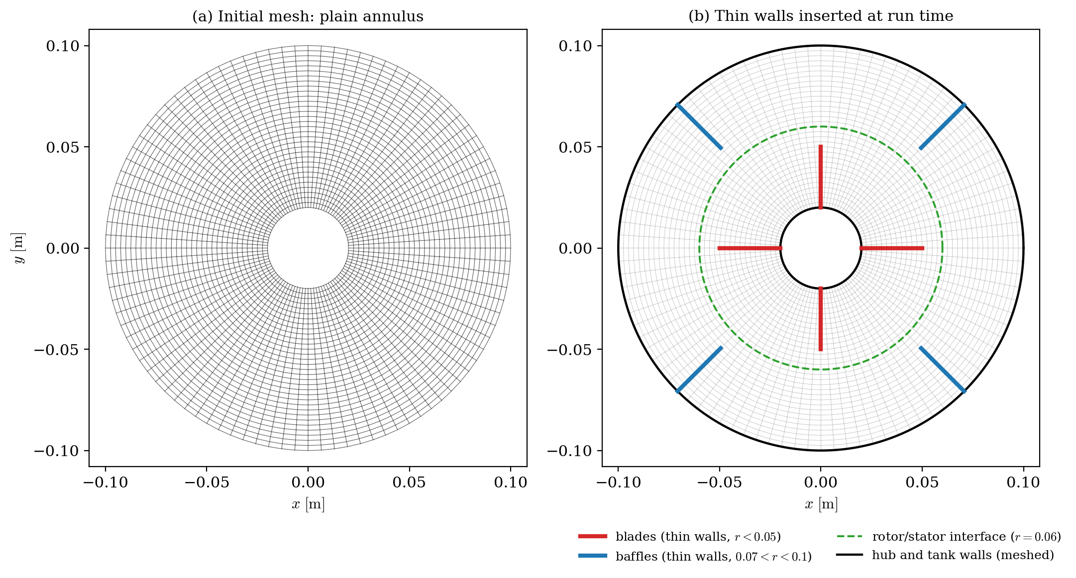
Figure 1: (a) the mesh as read from mixerVessel2D.msh: a plain annulus, with no obstacle inside. (b) the blades (red) and baffles (blue) inserted at run time as thin walls; the dashed green circle is the rotor/stator interface, which is not a wall but the limit of the rotating zone.

Thin walls

The blades and baffles are not meshed (Figure 1a): they are created at run time by a mesh preprocessing operation that turns interior faces selected by geometric criteria into pairs of coincident boundary faces (Figure 1b). In the GUI, open Mesh → Preprocessing, tab Other, box Interior to boundary faces (boundary insertion): the Add button creates one row per insertion, and each row holds one selection criterion. For instance the row creating the two blades lying along the \(x\) axis reads:

plane[0, 1, 0, 0, 0.001] and cylinder[0, 0, -1, 0, 0, 1, 0.05]

that is: interior faces within \(0.001\) m of the plane \(y = 0\), inside the cylinder of radius \(0.05\) m. This is a convenient way to add zero-thickness internal obstacles to an existing mesh.

Note that the insertion itself is a pure mesh operation, performed before the boundary conditions are applied: it does not decide the boundary condition of the new faces. The inserted faces carry no group name (the zone id column of the GUI table is only a row counter), so they belong to no boundary zone, and code_saturne then applies its default condition: smooth wall. This is exactly what blades and baffles require, so this setup adds nothing: the boundary conditions section simply ignores these faces. If another nature were needed (a symmetry would make the obstacles slip walls, for instance), one would define a boundary zone whose selection criterion catches the inserted faces, e.g. the same geometric criterion, or not (2 or 3 or 4 or 5) (all boundary faces outside the four mesh groups); keep in mind that such a criterion catches both coincident faces of each inserted pair.

Boundary conditions

Boundary	Location	Nature	Zone selector
walls	hub + tank wall	Smooth wall (no-slip)	4 or 5
z0, z1	spanwise planes	Symmetry	2, 3
(thin walls)	blades + baffles	Smooth wall (default, no zone defined)	(none)

Note on gmsh meshes: code_saturne selects boundary zones of a .msh file by the numeric physical tags (here 2, 3, 4, 5), not by the physical names (z0, z1, hub, tank_wall).

Numerical setup

Setting	Value	Rationale
Turbomachinery model	Frozen rotor	Steady rotor-stator approximation
Rotor zone	cylinder[0, 0, -0.1, 0, 0, 0.1, 0.06]	Cells with \(r < 0.06\) m rotate
Velocity-pressure coupling	SIMPLEC	Standard segregated coupling
Time-stepping	Fixed \(\Delta t = 2 \times 10^{-3}\) s	Pseudo-transient march (mean CFL \(\approx 1.4\)); larger steps trigger a numerical oscillation in the blade-root corner cells
Iterations	\(500\) (\(t = 1\) s \(\approx 17\) rotor revolutions)	Steady state reached well within this budget (Figure 2)
Turbulence	k-ε Linear Production, scalable wall functions	Robust on the coarse near-wall mesh
Relaxation	\(0.3\) (pressure), \(0.5\) (velocity, \(k\), \(\varepsilon\))	Pseudo-steady convergence
Initialization	fluid at rest	The impeller spins the fluid up from rest

Running the simulation

The commands below start from the tutorial directory:

cd Tbm_Mixer_Vessel_2D/

Option A: Graphical interface

code_saturne gui CASE/DATA/setup.xml &

The GUI opens the pre-configured setup.xml. Review the setup if you wish, then launch the run with the gear (Run) button in the toolbar.

Option B: Command line

The command-line launcher is run from inside the case directory:

cd CASE

# serial
code_saturne run

# parallel (e.g. 2 MPI ranks)
code_saturne run --n 2

Each run creates a time-stamped directory CASE/RESU/<YYYYMMDD-HHMM>/ containing:

• run_solver.log: solver log (check the boundary faces type table: 448 wall faces including the thin walls, 6144 symmetry faces, 0 undefined),
• monitoring/probes_*.csv: probe histories,
• postprocessing/: volume fields in EnSight Gold format.

Results

Convergence

Four probes monitor the velocity magnitude at representative locations: the impeller jet just beyond the blade tips (\(r = 0.055\) m), the stator side of the rotor/stator interface (\(r = 0.065\) m), the near wake of a baffle (\(r = 0.085\) m), and a blade-root corner cell (\(r = 0.024\) m), the most numerically sensitive point of the case.

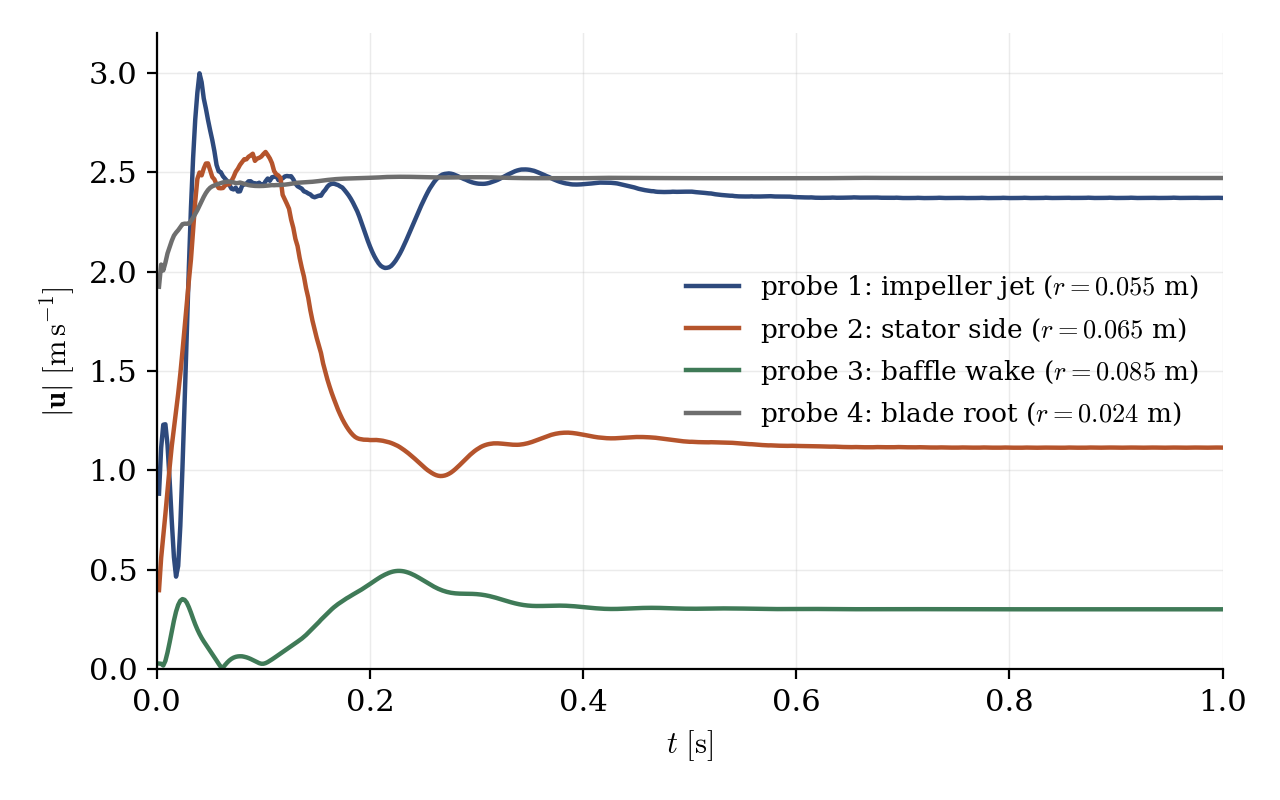
Figure 2: Velocity magnitude at the four monitoring probes. After the spin-up transient (about 0.4 s, i.e. 7 rotor revolutions), all probes settle on a strictly flat plateau: the frozen-rotor steady state is reached. The blade-root probe converges to $2.47\ \mathrm{m\,s^{-1}}$, the local entrainment velocity $\omega r$.

Velocity field

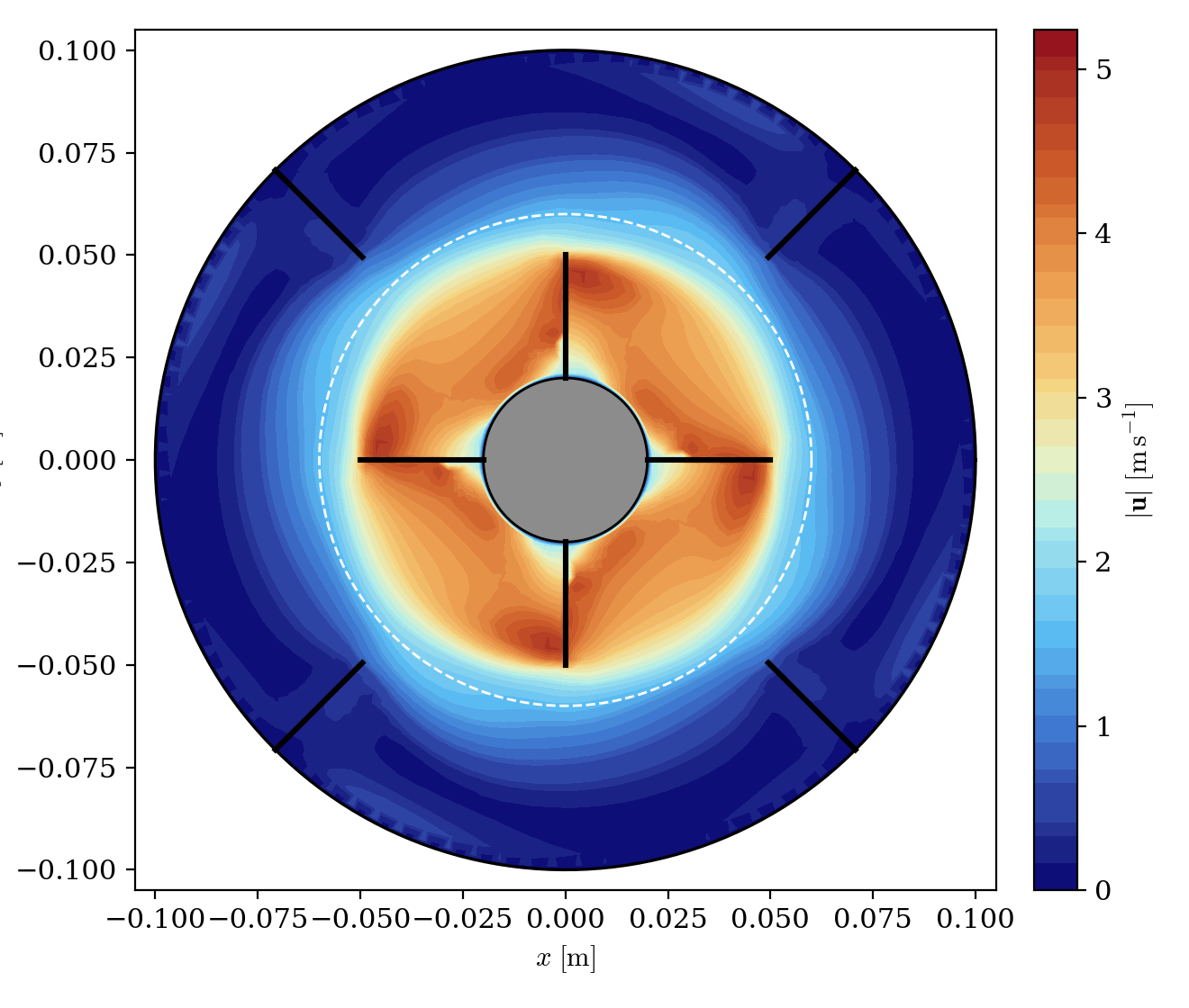
Figure 3: Velocity magnitude at convergence. The four blades (thick lines, $r < 0.05$ m) drive the rotating core; the white dashed circle is the rotor/stator interface ($r = 0.06$ m); the four baffles ($0.07 < r < 0.1$ m) hold the outer region nearly still, which is precisely their role in a stirred tank. The maximum velocity, $4.85\ \mathrm{m\,s^{-1}}$, stays below the blade tip speed of $5.24\ \mathrm{m\,s^{-1}}$.

The solution shows the expected stirred-tank pattern: a nearly solid-body rotating core carried by the impeller, thin high-speed jets leaving the blade tips, and an outer region kept almost at rest by the baffles. Keep in mind the frozen-rotor caveat: the steady solution depends on the angular position at which the rotor is frozen (here, blades at \(45°\) from the baffles); a transient rotor-stator computation would resolve the actual blade-passing dynamics.

Summary

This tutorial computed a baffled stirred tank with the frozen rotor model of code_saturne: rotor zone defined by a geometric criterion, blades and baffles inserted as zero-thickness thin walls into a plain annular mesh, k-ε Linear Production turbulence with scalable wall functions, and a relaxed SIMPLEC pseudo-transient monitored by four probes until a strictly steady state.

References

• code_saturne documentation
• E.L. Paul, V.A. Atiemo-Obeng, S.M. Kresta (eds). Handbook of Industrial Mixing: Science and Practice, Wiley, 2004.

Authors

Simvia - Questions, remarks and requests are welcome.