Two-Material Bar (Voltage Divider)
A step-by-step tutorial extending Elec_Joule_Bar: the same conducting bar, now made of two materials in series (\(\sigma_1 = 100\), \(\sigma_2 = 25\ \mathrm{S/m}\)). The case demonstrates that the electrical conductivity is a field (the industrial use of the Joule module: electrode regions and melts with different, temperature-dependent conductivities), and everything remains closed-form: the bar is a textbook voltage divider. It also teaches a classic finite-volume lesson along the way: the harmonic face average for discontinuous diffusivities.
Maintained by Simvia, part of the tutoriel-code_saturne collection.
Learning objectives
After completing this tutorial you will be able to:
- Prescribe a spatially variable electrical conductivity (a field filled in
cs_user_physical_properties.cpp). - Use the harmonic face interpolation of a discontinuous diffusivity (
imvisf), and know why the default arithmetic average biases the interface conductance. - Read the electric fields at a material interface: continuous current, jumping electric field.
Prerequisites
| Requirement | Detail |
|---|---|
| code_saturne | v9.1 |
| Case | Elec_Joule_Bar (the single-material bar, and the three user-file requirements of the Joule variant) |
If code_saturne is not yet installed, build it from the official homepage, pull a ready-to-use Singularity image from the Open Simulation Center, or pull the Simvia Docker image before continuing.
Case files
Elec_Two_Materials/
├── CASE/
│   ├── DATA/
│   │   └── setup.xml                        # identical to Elec_Joule_Bar
│   └── SRC/
│       ├── cs_user_physical_properties.cpp  # sigma(x) field + T(H) law
│       ├── cs_user_boundary_conditions.cpp  # electrode potentials (see Elec_Joule_Bar)
│       └── cs_user_parameters.cpp           # harmonic face average for sigma
├── FIGURES/                                 # figures used in this README
└── README.md
There is no MESH directory: the mesh is generated at run time by the built-in cartesian mesher. The
setup.xmlis strictly identical to the single-material case: the whole difference lives in the user routines.
Physical model
The bar of Elec_Joule_Bar (\(100 \times 20 \times 5\) mm, \(U = 10\) V across) is split at mid-length into two materials. In series, the current density is continuous and the bar behaves as a voltage divider; everything follows from \(R_i = L_i/(\sigma_i A)\):
| Quantity | Exact value |
|---|---|
| Resistances | \(R_1 = 5\ \Omega\), \(R_2 = 20\ \Omega\) |
| Current | \(I = U/(R_1+R_2) = 0.4\) A (\(J = 4000\ \mathrm{A/m^2}\), continuous) |
| Electric field | \(E_1 = 40\), \(E_2 = 160\ \mathrm{V/m}\): jump ratio \(= \sigma_1/\sigma_2 = 4\) |
| Interface potential | \(\phi = 2\) V (piecewise-linear \(\phi\)) |
| Dissipations | \(q_1 = 1.6 \times 10^5\), \(q_2 = 6.4 \times 10^5\ \mathrm{W/m^3}\); \(P = UI = 4\) W |
| Thermal parabolas | \(\Delta T_{max} = 0.8\) K (\(\sigma_1\) side), \(3.2\) K (\(\sigma_2\) side) |
The harmonic average lesson
The conductivity jumps across a single face. With the default arithmetic face average of the diffusivity, the interface conductance is overestimated, and the computed current comes out \(0.7\%\) too high on this mesh (the error decreases with refinement, but slowly). The classic finite-volume remedy is the harmonic average, which reproduces resistances in series exactly: with imvisf = 1 on the potential equation (set in cs_user_parameters.cpp), the computed plateaus land on \(E_1 = 40.0\) and \(E_2 = 160.\ \mathrm{V/m}\) and the interface potential on \(2.0\) V. The same option matters for any transported quantity with a discontinuous diffusivity: multi-material conduction, conjugate heat transfer.
Flow parameters
| Quantity | Symbol | Value | Source |
|---|---|---|---|
| Conductivities | \(\sigma_1\), \(\sigma_2\) | \(100\), \(25\ \mathrm{S/m}\) (\(x \lessgtr 50\) mm) | cs_user_physical_properties.cpp |
| Potential difference | \(U\) | \(10\) V | cs_user_boundary_conditions.cpp |
| Face interpolation of \(\sigma\) | imvisf |
harmonic | cs_user_parameters.cpp |
| Material (thermal) | \(\rho\), \(c_p\), \(\lambda\) | \(1000\), \(100\), \(10\) (SI) | fluid_properties |
| Bar, mesh, time | as in Elec_Joule_Bar | setup.xml |
Geometry and boundary conditions
Identical to Elec_Joule_Bar: electrodes at the ends (\(\phi = 0\) and \(10\) V, adiabatic), cooled lateral walls (\(T_w = 300\) K, electrically insulated), symmetry on the spanwise planes. The material interface at \(x = 50\) mm is not a boundary: it exists only through the \(\sigma\) field.
Numerical setup
As in Elec_Joule_Bar, plus the harmonic face interpolation of the potential diffusivity (see above).
Running the simulation
The commands below start from the tutorial directory:
cd Elec_Two_Materials/
Option A: Graphical interface
code_saturne gui CASE/DATA/setup.xml &
The GUI opens the pre-configured setup.xml. Review the setup if you wish,
then launch the run with the gear (Run) button in the toolbar.
Option B: Command line
The command-line launcher is run from inside the case directory:
cd CASE

# serial (a few seconds)
code_saturne run
The three user routines are compiled automatically at the beginning of the run.
Results
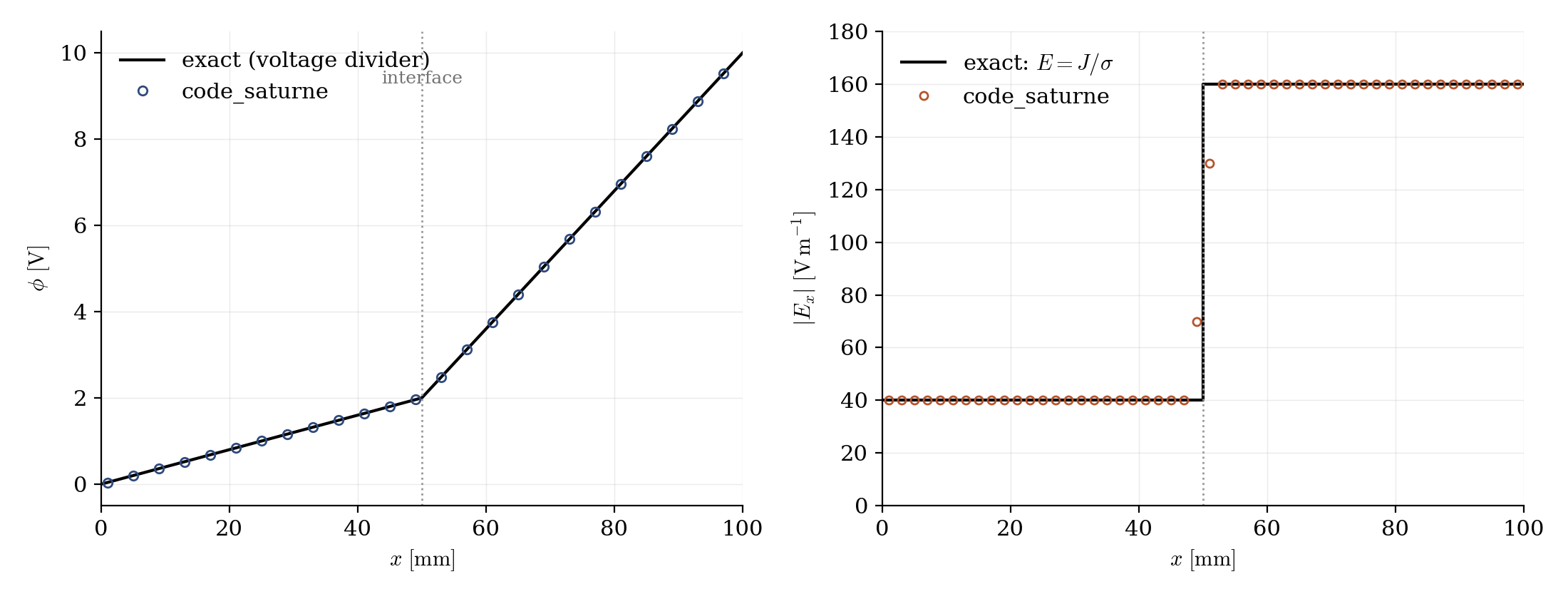
Figure 1: left, the potential is piecewise linear with the exact interface value ($2.0$ V computed); right, the electric field jumps by the conductivity ratio ($40.0$ and $160.\ \mathrm{V/m}$ computed on the plateaus). The one point inside the interface cell pair reflects the cell-gradient reconstruction across the kink of $\phi$, not the solution itself.
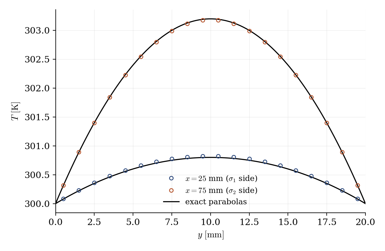
Figure 2: temperature across the bar at the quarter lengths: each half carries its own parabola, with maxima in the dissipation ratio $q_2/q_1 = 4$ ($0.83$ and $3.18$ K computed for $0.8$ and $3.2$ K expected: the small deviations are the longitudinal conduction between the two halves, absent from the 1D formula).
One post-processing caveat: the cell-averaged current and Joule power include the two cell layers straddling the potential kink, where the reconstructed gradient is smeared; integral values quoted from these fields come out \(\approx 1\%\) high. The solution itself is exact, as the plateaus and the interface potential show.
Summary
This tutorial turned the electrical conductivity into a field: two materials in series make the bar a textbook voltage divider, computed exactly (plateaus \(40./160.\ \mathrm{V/m}\), interface at \(2.0\) V) once the harmonic face average of the discontinuous diffusivity is enabled: a one-line numerical option worth knowing far beyond the electric module. Each half then heats with its own dissipation, giving two thermal parabolas in ratio four.
References
- S.V. Patankar. Numerical Heat Transfer and Fluid Flow, Hemisphere, 1980 (section 4.2-3: the harmonic mean for discontinuous conductivities).
- code_saturne documentation
Authors
Simvia - Questions, remarks and requests are welcome.