Cavitating Throttle (VOF Cavitation Model)
A step-by-step tutorial for simulating cavitation with the VOF cavitation model (Merkle) of code_saturne: the pressure drop through a small 2D throttle (orifice) creates a steady vapor pocket in which the pressure locks onto the saturation pressure. The case teaches the complete cavitation workflow, including the one mandatory user routine without which the model silently produces no vapor at all.
Maintained by Simvia, part of the tutoriel-code_saturne collection.
Learning objectives
After completing this tutorial you will be able to:
- Enable the cavitation model (VOF homogeneous mixture with Merkle mass-transfer source terms).
- Set the mandatory model parameters (
presat,uinf,linf) incs_user_parameters.cpp, and understand why the run produces no vapor at all without this file. - Size a cavitating case with the cavitation number, using the system pressure as the control knob (as in a cavitation tunnel).
- Monitor the health of a cavitating run (VOF mass balance, void-fraction clipping messages).
Prerequisites
| Requirement | Detail |
|---|---|
| code_saturne | v9.1 |
| Case | Vof_Kelvin_Helmholtz (basics of the VOF model) |
If code_saturne is not yet installed, build it from the official homepage, pull a ready-to-use Singularity image from the Open Simulation Center, or pull the Simvia Docker image before continuing.
Case files
Vof_Cavitating_Throttle/
├── CASE/
│   ├── DATA/
│   │   └── setup.xml                # pre-configured GUI case
│   └── SRC/
│       └── cs_user_parameters.cpp   # cavitation model parameters (MANDATORY)
├── MESH/
│   └── throttle.med                 # 2D throttle mesh, 7710 hexahedra
├── FIGURES/                         # figures used in this README
└── README.md
Physical model
The cavitation model of code_saturne is the VOF homogeneous mixture model with mass transfer: one set of incompressible momentum equations for the mixture, one transport equation for the void fraction \(\alpha\) (vapor volume fraction), and a Merkle source term \(\Gamma_v\) that vaporizes liquid where the pressure drops below the saturation pressure \(p_{\mathrm{sat}}\) and condenses vapor where it rises back above:
The Merkle source terms are proportional to \(\min(p - p_{\mathrm{sat}}, 0)\) (vaporization) and \(\max(p - p_{\mathrm{sat}}, 0)\) (condensation), with empirical constants and a time scale built from the model reference velocity and length (\(u_\infty\), \(\ell_\infty\)).
The classic signature of cavitation, visible in the results below: wherever the vapor pocket sits, the source terms drive the local pressure to lock onto \(p_{\mathrm{sat}}\).
The single most important file: cs_user_parameters.cpp
The cavitation model parameters are not exposed in the GUI: they can only be set in cs_user_parameters.cpp. If you activate the cavitation model in the GUI and do not provide this file, the run proceeds normally but no vapor is ever created: the model reference velocity uinf keeps an unset sentinel value which makes the source terms numerically zero. This is the single most common cavitation setup mistake. The shipped file sets:
presat = 2340Pa: saturation pressure of water at 20 °C. It is compared to the total (absolute) pressure, which includes the reference pressure \(P_0\) set in the GUI;uinf = 21m/s,linf = 2e-3m: bulk velocity in the throat and throat length, which calibrate the vaporization/condensation time scale (\(t_\infty = \ell_\infty/u_\infty\));- the empirical constants
cdest,cprodkeep their defaults.
Sizing: the cavitation number
Whether and how much a device cavitates is governed by the cavitation number, built here on the throat velocity \(U_t\):
This case controls \(\sigma\) through the system pressure, exactly as a laboratory cavitation tunnel does: the outlet is held at \(P_0 = 81325\) Pa (0.80 atm absolute) rather than atmospheric. With water at 20 °C everywhere (\(\rho_l\), \(\mu_l\), \(p_{\mathrm{sat}}\) all consistent), this places the operating point in a steady, bounded pocket regime: the depression peak of the developed flow exceeds the cavitation threshold by a controlled margin (about 10 kPa). Two pitfalls of sizing such a case on a coarse mesh, found the hard way while building it, are worth recording: the suction peak at the throat corners is smeared by the mesh (it grows far more slowly with the inlet velocity than the ideal \(U^2\) scaling suggests), and an operating point marginally above the threshold produces a bistable, non-reproducible flow in which the vapor pocket created by the impulsive start may or may not survive. Size for a clear margin, on the knob that acts directly on the threshold.
Flow parameters
| Quantity | Symbol | Value | Source |
|---|---|---|---|
| Liquid (water, 20 °C) | \(\rho_l\), \(\mu_l\) | \(998\ \mathrm{kg\,m^{-3}}\), \(10^{-3}\ \mathrm{Pa\,s}\) | density, molecular_viscosity (value_0) |
| Vapor | \(\rho_v\), \(\mu_v\) | \(1\ \mathrm{kg\,m^{-3}}\), \(10^{-5}\ \mathrm{Pa\,s}\) | (value_1) |
| Saturation pressure | \(p_{\mathrm{sat}}\) | \(2340\) Pa (absolute) | cs_user_parameters.cpp |
| System (outlet) pressure | \(P_0\) | \(81325\) Pa (0.80 atm) | reference_pressure |
| Inlet velocity | \(U_{in}\) | \(1.2\ \mathrm{m\,s^{-1}}\) | inlet/velocity_pressure/norm |
| Throat velocity | \(U_t\) | \(\approx 24.6\ \mathrm{m\,s^{-1}}\) | computed |
| Cavitation number | \(\sigma\) | \(\approx 0.26\) | derived |
| Time step | \(\Delta t\) | \(2 \times 10^{-6}\) s (fixed, CFL \(\approx 0.5\)) | time_step_ref |
| Simulated time | \(t_{end}\) | \(50\) ms (\(25000\) steps) | iterations |
Geometry and boundary conditions
The geometry is the throttle of Winklhofer et al. (2001): a channel of height \(5\) mm and length \(17\) mm, restricted by a throat of height \(0.3\) mm and length \(2\) mm (\(x = 5\) to \(7\) mm). The mesh (MESH/throttle.med) has \(7710\) hexahedra, one cell thick, with only 3 cells across the throat: this is a deliberately coarse, minimal case (about 10 minutes on 4 cores).
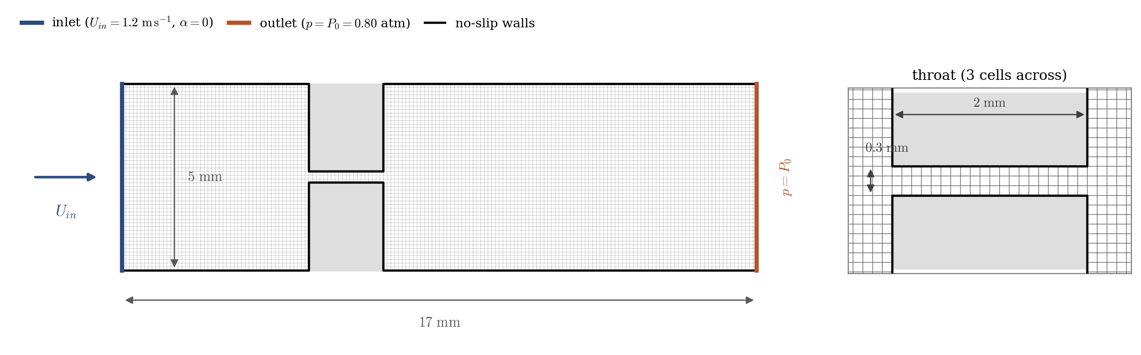
Figure 1: computational domain and mesh. Velocity inlet (blue), pressure outlet at the system pressure $P_0$ (orange), no-slip walls (black); the spanwise planes (not shown) carry the symmetry condition. Right: zoom on the throat and its 3 cells across.
| Boundary | Location | Nature | Prescribed value | Zone selector |
|---|---|---|---|---|
Inlet |
left | Velocity inlet | \(1.2\ \mathrm{m\,s^{-1}}\), \(\alpha = 0\) | inlet |
Outlet |
right | Free outlet | \(p = P_0\) | outlet |
Walls |
channel + throat walls | Smooth wall | (none) | walls |
Sym |
spanwise planes | Symmetry | (none) | not (inlet or outlet or walls) |
Numerical setup
| Setting | Value | Rationale |
|---|---|---|
| Two-phase model | VOF + Merkle cavitation (merkle_model) |
Mass transfer between phases |
| Velocity-pressure coupling | SIMPLEC | Standard segregated coupling |
| Velocity convection scheme | 1st-order upwind (blending_factor 0) |
Robustness on the coarse mesh |
| Gradients | Iterative (Green) | Default, robust |
| Time-stepping | Fixed \(\Delta t = 2 \times 10^{-6}\) s | Time-accurate transient, CFL \(\approx 0.5\) |
| Turbulence | none (laminar) | The point is the cavitation model |
| Initialization | fluid at rest, \(\alpha = 0\) | Impulsive start |
Running the simulation
The commands below start from the tutorial directory:
cd Vof_Cavitating_Throttle/
Option A: Graphical interface
code_saturne gui CASE/DATA/setup.xml &
The GUI opens the pre-configured setup.xml. Review the setup if you wish,
then launch the run with the gear (Run) button in the toolbar.
Option B: Command line
The command-line launcher is run from inside the case directory:
cd CASE

# serial
code_saturne run

# parallel (e.g. 4 MPI ranks)
code_saturne run --n 4
The user routine SRC/cs_user_parameters.cpp is compiled automatically at the beginning of the run.
Each run creates a time-stamped directory CASE/RESU/<YYYYMMDD-HHMM>/ containing:
run_solver.log: solver log,monitoring/probes_*.csv: throat probe histories,postprocessing/: time series of volume fields in EnSight Gold format.
Two log messages deserve a comment. Warnings about void-fraction clipping are expected in cavitating runs (the min/max principle criterion is dominated by the worst near-empty cell; violations are handled by clipping). The health indicator to watch instead is the VOF model, mass balance line: transient spikes while the vapor structures develop, then back to round-off level (\(\sim 10^{-11}\) kg/s here) once the pocket is steady.
Results
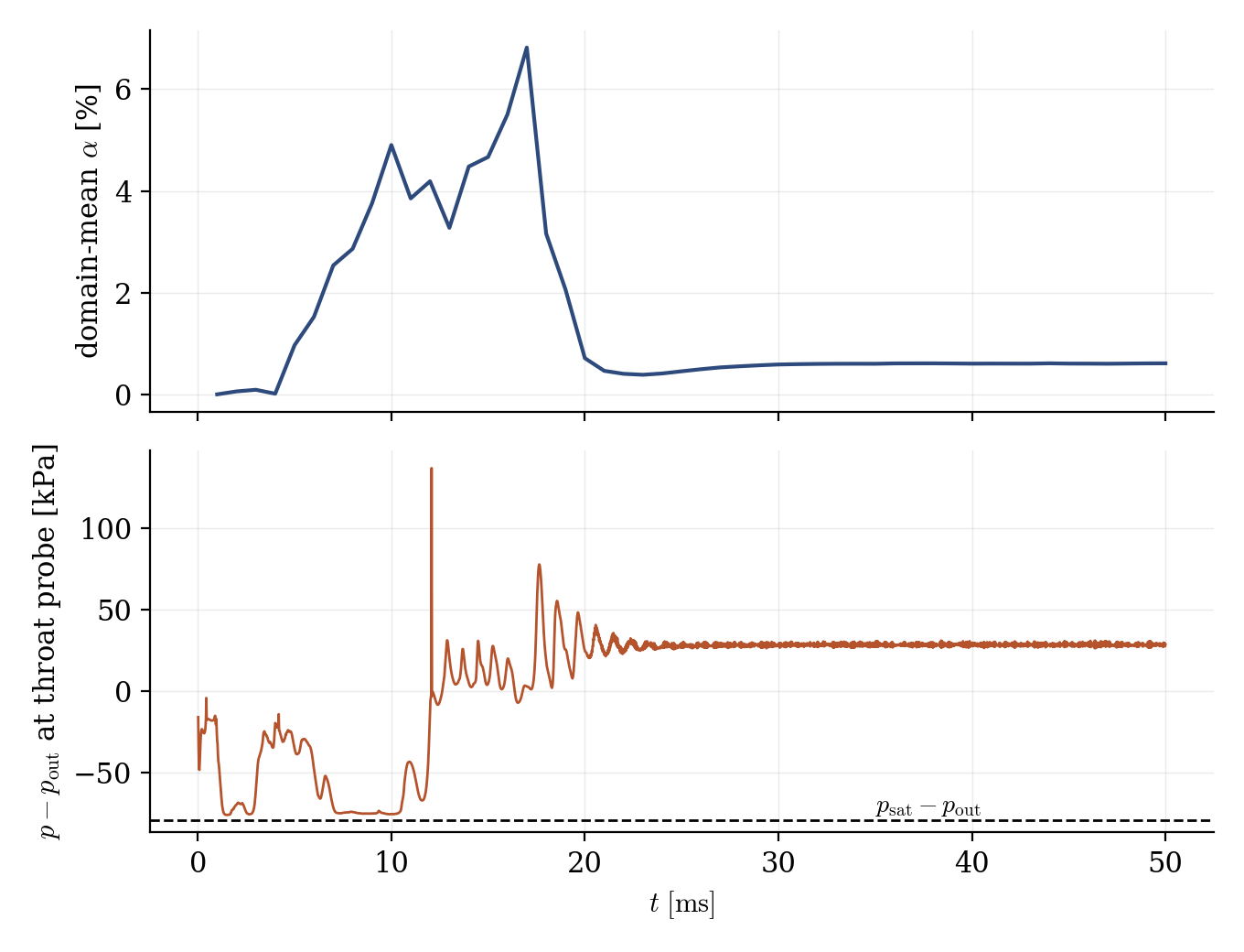
Figure 2: time histories. Top: domain-mean void fraction; the impulsive start triggers a large transient vapor burst (up to 7% of the domain), which collapses around $t = 20$ ms, after which the flow settles onto a steady bounded pocket (flat plateau to the end of the run). Bottom: pressure at the throat-axis probe; during the burst the probe reads the saturation pressure (dashed line), then settles with the steady flow.
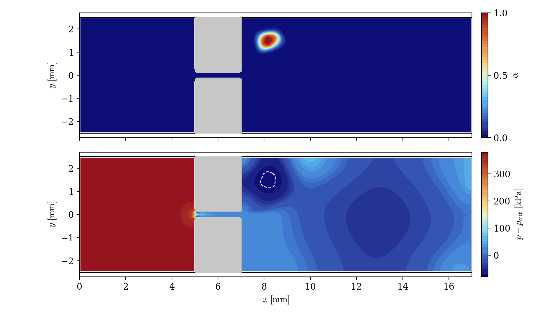
Figure 3: fields at $t = 50$ ms. Top: void fraction; the steady vapor pocket ($\alpha \approx 1$) sits in the recirculation eddy of the sudden expansion, on the side the jet detaches from (the jet issuing from the throat attaches to one wall, a Coanda effect classical in sudden expansions). Bottom: pressure; inside the pocket the pressure locks onto $p_{\mathrm{sat}}$ (white dashed contour; computed minimum $-79014$ Pa vs. $p_{\mathrm{sat}} - P_0 = -78985$ Pa, i.e. 0.04%).
Summary
This tutorial computed a cavitating throttle with the VOF cavitation model (Merkle) of code_saturne: model activated in the GUI but parameterized by the mandatory cs_user_parameters.cpp (presat, uinf, linf), operating point sized through the cavitation number with the system pressure as control knob, and a steady bounded vapor pocket whose internal pressure locks onto the saturation pressure to within 0.04%.
References
- E. Winklhofer, E. Kull, E. Kelz, A. Morozov. Comprehensive hydraulic and flow field documentation in model throttle experiments under cavitation conditions, ILASS-Europe, 2001.
- C.L. Merkle, J. Feng, P.E.O. Buelow. Computational modeling of the dynamics of sheet cavitation, 3rd Int. Symp. on Cavitation, 1998.
- code_saturne documentation
Authors
Simvia - Questions, remarks and requests are welcome.