Inviscid Hydrofoil¶

Browse this case on GitHub

A step-by-step tutorial for simulating the incompressible, inviscid flow through a 2D channel around a NACA 0012 hydrofoil using code_saturne. The case is a showcase to get familiar with code_saturne.

Maintained by Simvia, part of the tutoriel-code_saturne collection.

Learning objectives¶

After completing this tutorial you will be able to:

Set up a steady, incompressible inviscid simulation in code_saturne from the GUI.
Apply inlet, outlet and symmetry (slip-wall) boundary conditions on an unstructured triangular mesh.
Drive a steady solution with local (pseudo) time-stepping and the SIMPLEC coupling.
Run the case in serial or parallel and locate the solver outputs (log, probes, EnSight fields).

Prerequisites¶

Requirement	Detail
code_saturne	v9.1
Background	Basic notions of incompressible aerodynamics and potential (inviscid) flow theory

If code_saturne is not yet installed, build it from the official homepage, pull a ready-to-use Singularity image from the Open Simulation Center, or pull the Simvia Docker image before continuing.

Case files¶

Inc_Inviscid_Hydrofoil/
├── CASE/
│   ├── DATA/
│   │   └── setup.xml          # pre-configured GUI case
│   └── SRC/
│       └── cs_user_extra_operations.cpp   # user routine: computes lift/drag coefficients (Cl, Cd)
├── MESH/
│   └── mesh_NACA0012_5deg_6814.msh
├── FIGURES/                   # figures used in this README
└── README.md

Physical model¶

The flow is steady, incompressible and inviscid, governed by the Navier-Stokes equations which are simplified to obtain Euler Equations:

\[ \nabla\cdot\mathbf{u}=0,\qquad \rho\,(\mathbf{u} \cdot \nabla)\,\mathbf{u} = -\nabla p \]

The case is run with the incompressible solver, which is the natural choice for this low-speed flow ($U_\infty=1.775\ \mathrm{m\,s^{-1}}$, Mach number effectively zero), with $\mu\to 0$ the viscous term vanishes entirely.

Flow parameters¶

Quantity	Symbol	Value	Source in `setup.xml`
Density	$\rho$	$998.2\ \mathrm{kg\,m^{-3}}$	`physical_properties/density`
Dynamic viscosity	$\mu$	$1e-12\ \mathrm{Pa\,s}$	`molecular_viscosity` ~negligible
Kinematic viscosity	$\nu=\mu/\rho$	$1.001e-15\ \mathrm{m^2\,s^{-1}}$	derived & negligible
Mean inlet velocity	$U_\infty$	$1.775\ \mathrm{m\,s^{-1}}$	`inlet/velocity_pressure/norm_formula`
Chord (reference length)	$c$	$1\ \mathrm{m}$	(geometry)
Reynolds number	$Re_c$	$\infty$	(see below)

The Reynolds number is recovered directly from the prescribed properties:

\[ Re_c=\frac{\rho\,U_\infty\,c}{\mu} =\frac{998.2\times 1.775\times 1}{\mu\to 0}\to\infty. \]

Geometry and boundary conditions¶

The domain is a water channel featuring a NACA 0012 hydrofoil in the centre. The channel is $20c$ wide and $12c$ high, where $c=1\ \mathrm{m}$ is the airfoil chord, the mesh extends over $x\in[-10,10]$, $y\in[-6,6]$ and a single cell in $z\in[0,1]$. The hydrofoil is inclined at about 5 degrees angle of attack relative to the parallel channel walls. The two spanwise ($xy$) planes carry a symmetry condition, so the computation is effectively two-dimensional. The upper and lower walls and the foil surface are also assigned a symmetry (slip-wall) boundary condition, enforcing zero normal velocity and zero wall shear stress, consistent with an inviscid, zero-viscosity flow assumption.

Boundary	Location	Nature	Prescribed value	Zone id
`inlet`	left ($x=-10$)	Inlet	$U_\infty=1.775\ \mathrm{m\,s^{-1}}$ (mean)	100
`outlet`	right ($x=+10$)	Outlet	$\partial\mathbf{u}/\partial n=0$, $p$ Dirichlet	200
`body`	hydrofoil surface (centre)	Symmetry (slip)	(none)	1000
`wall1`	bottom ($y=-6$)	Symmetry (slip)	(none)	1001
`wall2`	top ($y=+6$)	Symmetry (slip)	(none)	1002
`sym1`	spanwise plane ($z=0$)	Symmetry	(none)	600
`sym2`	spanwise plane ($z=1$)	Symmetry	(none)	601

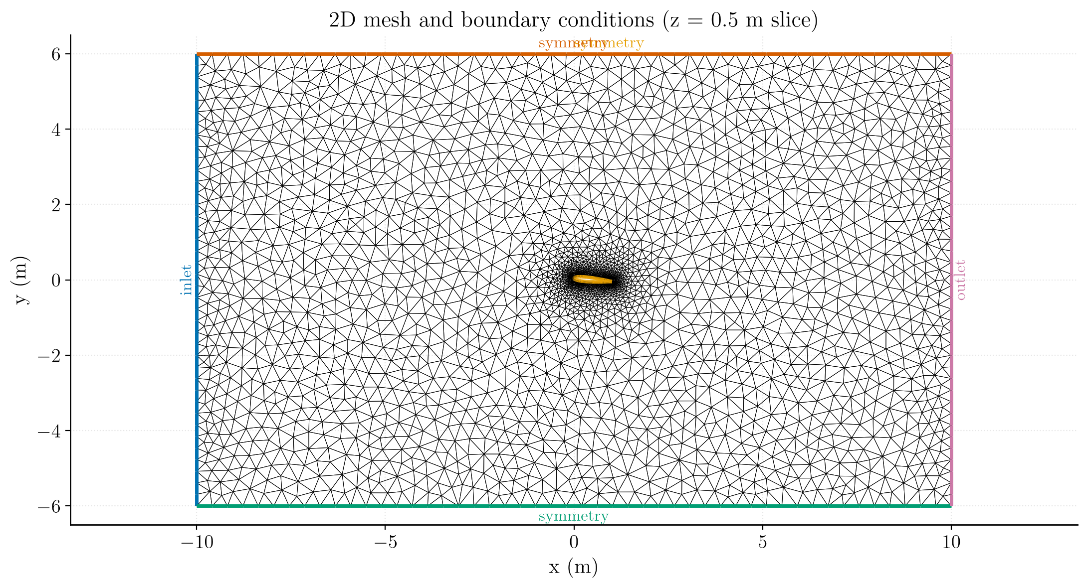
2D mesh of the Inviscid flow over the hydrofoil in the water channel colored by boundary condition: inlet (blue), outlet (pink), symmetry (slip wall) in all other faces.
Figure 1: Mesh and boundary conditions (z = 0.5 m slice): inlet (blue), outlet (pink), and symmetry (green/yellow/orange).

The computational mesh for the inviscid hydrofoil is composed of 6814 triangles with 3559 vertices per 2D plane (7118 vertices in the extruded mesh), 128 edges along the airfoil, and 49 edges along the upper and lower walls of the channel. The two spanwise planes (sym1/sym2) carry a symmetry condition, so the computation is effectively two-dimensional.

Numerical setup¶

Setting	Value	Rationale
Velocity-pressure coupling	SIMPLEC	Robust segregated coupling for steady incompressible flow
Time-stepping	Local (pseudo) time step	Accelerates convergence to steady state by using a per-cell time step
Reference time step	$\Delta t_\mathrm{ref}=0.01\ \mathrm{s}$	Seed value, bounded by min/max factors $[0.1,\,1000]$
Max Courant number	1	Caps the local time step away from the wall
Iterations	2000	Steady state reached well within this budget
Initialization	$\mathbf{u}=(U_\infty,0,0)$	Freestream start with a norm user law in the inlet
Gradient reconstruction Type	Least squares	Full (all vertex adjacent)

Two monitoring probes track convergence inside the channel at ($x=0.034\ \mathrm{m}$, $y=0.097\ \mathrm{m}$) and ($x=0.80\ \mathrm{m}$, $y=0.015\ \mathrm{m}$). They are sensitive indicators of when the flow around the foil has reached steady state.

Running the simulation¶

The commands below start from the tutorial directory:

cd Inc_Inviscid_Hydrofoil/

Option A: Graphical interface¶

code_saturne gui CASE/DATA/setup.xml &

The GUI opens the pre-configured setup.xml. Review the setup if you wish, then launch the run with the gear (Run) button in the toolbar. To run in parallel, set the number of processes under Calculation management > Performance settings before launching.

Option B: Command line¶

The command-line launcher is run from inside the case directory:

cd CASE

# serial
code_saturne run

# parallel (e.g. 8 MPI ranks)
code_saturne run --n 8

This small 2D case runs comfortably in serial, parallel execution is optional.

Each run creates a time-stamped directory CASE/RESU/<YYYYMMDD-HHMM>/ containing:

run_solver.log: solver log and residual history,
monitoring/: probe time series (probes_*.csv),
postprocessing/: volume and boundary fields in EnSight Gold format.

Results and verification¶

The figures below show the converged fields in dimensionless form: the pressure coefficient $C_p=(p-p_\infty)/\tfrac12\rho U_\infty^2$ and the velocity magnitude normalized by the free stream, $U/U_\infty$. The reference $p_\infty$ is the undisturbed upstream static pressure.

Pressure coefficient field ($C_p$)¶

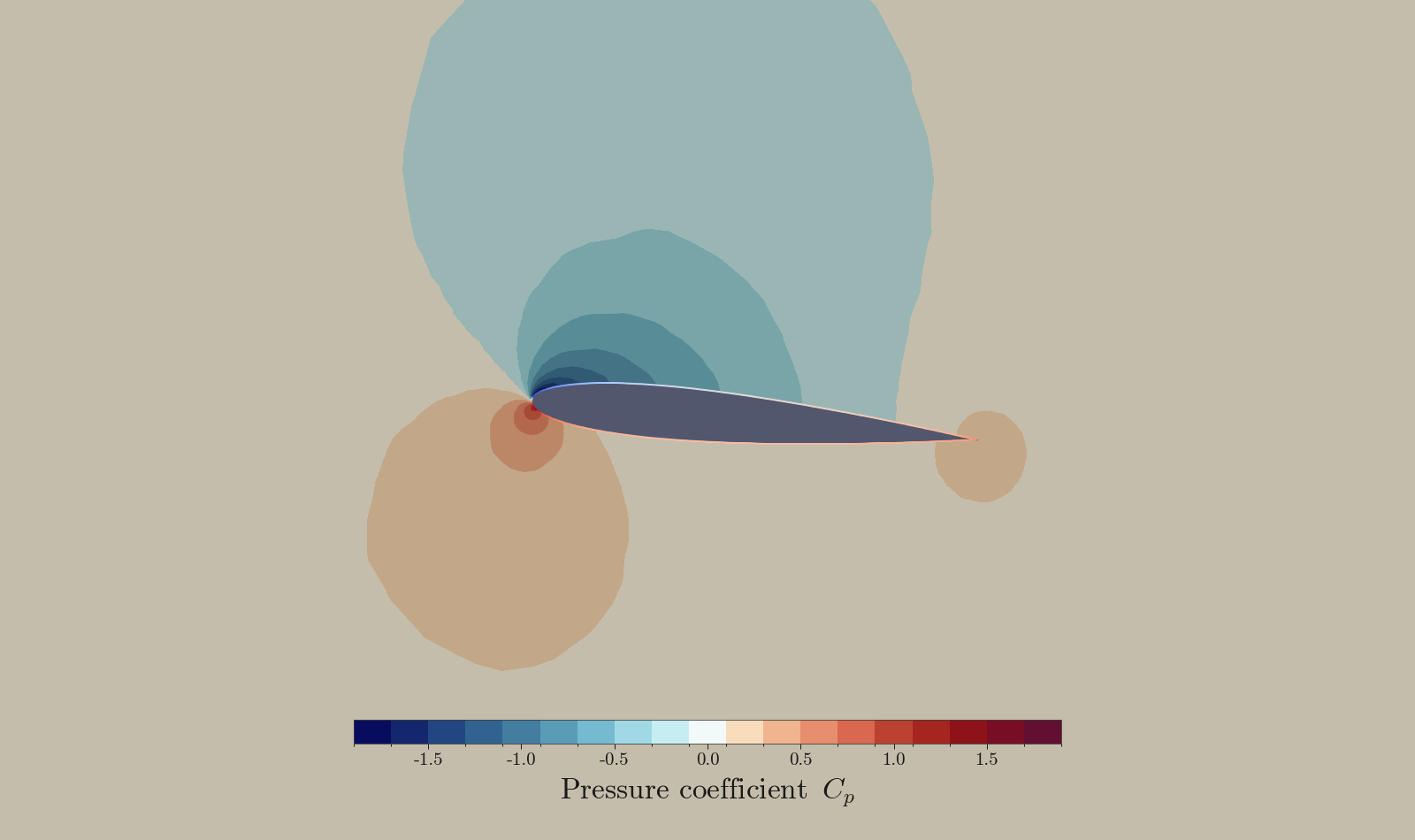
Pressure coefficient Cp field around the hydrofoil: leading-edge stagnation (Cp around 1) and suction (Cp around -1.9) over the upper surface, shown as filled contour bands.
Figure 2: Pressure-coefficient $C_p$ field - leading-edge stagnation ($C_p\approx 1$) and suction ($C_p\approx -1.9$) over the upper surface.

Normalized velocity field ($U/U_\infty$)¶

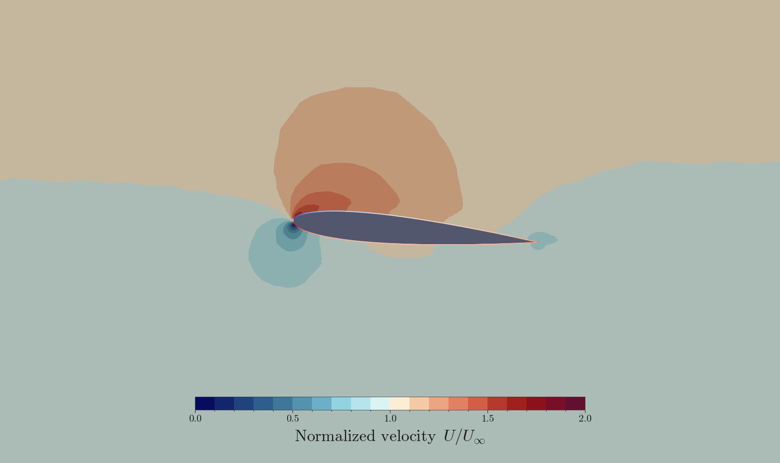
Normalized velocity field U over U-infinity around the hydrofoil: acceleration above the upper surface and near-zero velocity at the leading-edge stagnation point, shown as filled contour bands.
Figure 3: Normalized velocity $U/U_\infty$ field - acceleration over the upper surface ($U/U_\infty>1$) and the leading-edge stagnation point ($U/U_\infty\to 0$).

Pressure Coefficient Distribution (Cₚ) over a NACA 0012 Airfoil at α = 5°¶

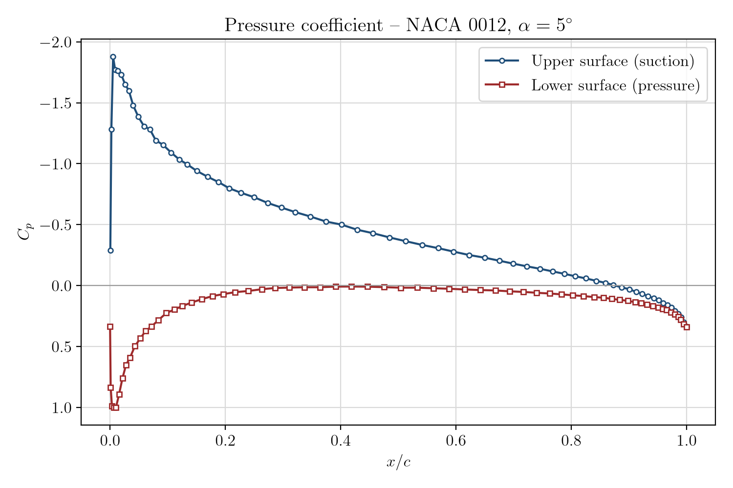
Pressure coefficient Cp along the chord on the upper and lower surfaces of the NACA 0012 at 5 degrees angle of attack.
Figure 4: Pressure coefficient $C_p$ along the chord ($x/c$) on the upper and lower surfaces of the NACA 0012 at $\alpha = 5°$.

This graph shows the pressure coefficient $C_p$ along the dimensionless chord ($x/c$) of the symmetric NACA 0012 airfoil. Two curves are plotted, one per surface:

Upper surface (suction side) - a peak near the leading edge at $C_p\approx-1.9$, characteristic of the accelerated flow over the upper surface. $C_p$ then gradually recovers (becomes less negative) toward the trailing edge, indicating flow deceleration. This low-pressure region is the primary contributor to lift.
Lower surface - starts at the leading edge near the stagnation value $C_p\approx 1$, then rises to slightly positive or near-zero values. The pressure on the lower surface stays generally higher than the freestream reference, contributing positively to lift.

Summary¶

This tutorial set up an incompressible, inviscid flow in a channel around a NACA 0012 hydrofoil in code_saturne. The computed $C_p$ distribution shows the expected leading-edge stagnation point and the suction peak on the upper surface, consistent with inviscid potential-flow theory for a NACA 0012 at $\alpha = 5°$. The user routine cs_user_extra_operations.cpp additionally reports the lift and drag coefficients ($C_l$, $C_d$) in lift_drag.csv. This case is a good starting point for more complex incompressible CFD simulations.

References¶

A viscous/inviscid interactive approach and its application to hydrofoils and propellers with non−zero trailing edge thickness Resource, Inviscid flow over an Hydrofoil
code_saturne documentation

Authors¶

Simvia - Questions, remarks and requests are welcome.