Neutral Atmospheric Boundary Layer: the Log Law (atmo)
A step-by-step tutorial for the atmospheric flows module (atmo) of
code_saturne: a neutral atmospheric boundary layer over flat, rough
terrain. The showcased feature is the atmospheric surface layer with a
rough-wall boundary (roughness length \(z_0\)): driven to equilibrium by a
constant pressure gradient, the mean wind settles into the logarithmic
profile that is the cornerstone of micrometeorology. It is the atmospheric
cousin of the turbulent channel:
same periodic, source-driven approach, but with a rough ground and validated
against the law of the wall for the atmosphere.
Maintained by Simvia, part of the tutoriel-code_saturne collection.
Learning objectives
After completing this tutorial you will be able to:
- Activate the atmospheric flows module in neutral mode
(
atmospheric_flows model="constant"). - Set a rough-wall ground boundary with a roughness length \(z_0\).
- Drive a constant-stress surface layer with a body force and fix the friction velocity \(u_*\) by the momentum balance.
- Validate the mean wind against the logarithmic law \(U(z) = (u_*/\kappa)\ln\big((z+z_0)/z_0\big)\).
Prerequisites
| Requirement | Detail |
|---|---|
| code_saturne | v9.1 |
| Tutorials | Inc_Turbulent_Channel (periodic, source-driven wall turbulence), Inc_Streamwise_Periodic |
If code_saturne is not yet installed, build it from the official homepage, pull a ready-to-use Singularity image from the Open Simulation Center, or pull the Simvia Docker image before continuing.
Case files
Atmo_Neutral_BoundaryLayer/
├── CASE/
│   ├── DATA/setup.xml                    # atmo model, k-epsilon, rough wall, periodicity
│   └── SRC/
│       ├── cs_user_source_terms.cpp      # constant streamwise body force
│       └── cs_user_initialization.cpp    # log-law initial guess (k, epsilon)
├── FIGURES/
└── README.md
No mesh file: the vertical slice is built by the built-in cartesian mesher.
Physical model
Close to the ground, in the absence of buoyancy (neutral stratification), the mean wind of the atmospheric surface layer follows the logarithmic law
with \(u_*\) the friction velocity, \(\kappa \approx 0.42\) the von Karman constant (code_saturne's value), and \(z_0\) the aerodynamic roughness length of the surface. The turbulent kinetic energy is roughly constant in the surface layer, \(k \approx u_*^2/\sqrt{C_\mu}\).
The domain is a vertical slice, periodic in the streamwise direction and capped by a symmetry plane. A constant horizontal body force \(f_x = \rho\,u_*^2/H\) drives the flow; at equilibrium it balances the ground shear stress, so the friction velocity is fixed by construction, \(u_* = \sqrt{f_x H/\rho}\) (exactly as the momentum source sets \(u_\tau\) in the turbulent channel). The ground is a rough wall of roughness \(z_0\); turbulence uses the standard \(k\)-\(\varepsilon\) model.
Flow parameters
| Quantity | Symbol | Value |
|---|---|---|
| Domain height | \(H\) | \(1000\) m |
| Roughness length | \(z_0\) | \(0.1\) m (grassland) |
| Friction velocity | \(u_*\) | \(0.4\) m/s |
| von Karman constant | \(\kappa\) | \(0.42\) |
| Air density | \(\rho\) | \(1.225\) kg/m³ |
| Turbulence model | \(k\)-\(\varepsilon\) |
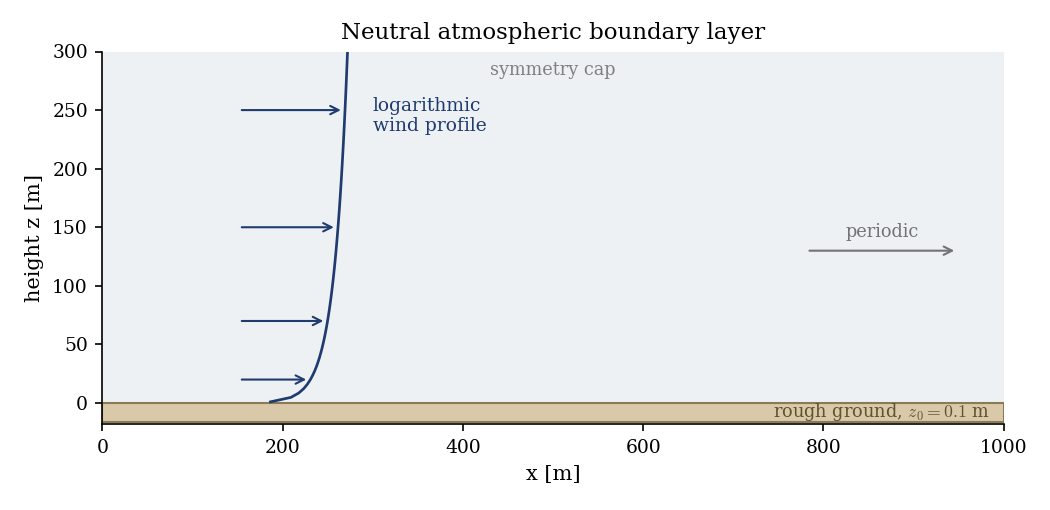
Figure 1: the neutral boundary layer. A body force drives the flow over a rough ground ($z_0$); the domain is streamwise periodic and capped by a symmetry plane.
Geometry and boundary conditions
The slice is \(1000\) m tall, graded so the cells are fine near the ground and
coarsen upward. The ground (ground, group Y0) is a rough wall with
\(z_0 = 0.1\) m; the top (Y1) and the spanwise sides (Z0, Z1) are symmetry
planes; the streamwise direction (X0/X1) is periodic.
Numerical setup
Neutral atmospheric model (\(k\)-\(\varepsilon\) turbulence), constant density. The
flow is advanced to a steady state (\(4000\) steps). cs_user_source_terms.cpp
applies the driving body force \(f_x = \rho u_*^2/H\); cs_user_initialization.cpp
starts the fields from the analytic log profile to speed convergence.
Running the simulation
cd CASE
code_saturne run --n 4
The mesh is generated internally. The run writes CASE/RESU/<id>/ with the
velocity, pressure and the turbulence fields \(k\) and \(\varepsilon\) in
postprocessing/.
Results and verification
Wind profile. Plotted against a logarithmic height axis, the computed mean wind is a straight line that lies on the analytic log law \(U(z) = (u_*/\kappa)\ln((z+z_0)/z_0)\) with \(u_* = 0.4\) m/s: the values agree to within one to two percent over the lower part of the domain (roughly \(z \approx 1\) to \(150\) m, about two decades). Higher up the wind runs a little faster than the pure log law, the expected effect of the shear stress falling toward the symmetry cap.
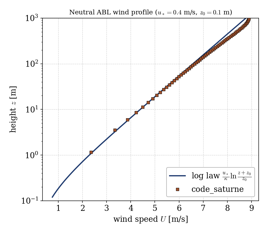
Figure 2: mean wind versus height. The code_saturne profile (symbols) follows the logarithmic law (line) over the lower part of the domain; the small deviation higher up follows the shear stress decreasing toward the symmetry cap.
The friction velocity itself is fixed exactly by the momentum balance, \(u_* = \sqrt{f_x H/\rho} = 0.4\) m/s, so the log law is a genuine prediction here, not a fitted curve: the roughness and the turbulence model together produce the profile.
Summary
This tutorial computed a neutral atmospheric boundary layer with the atmo
module: a rough ground and a driving pressure gradient produce a constant-stress
surface layer whose mean wind follows the logarithmic law, recovered to within a
couple of percent over two decades of height, with the friction velocity set by
the momentum balance. The lesson that carries beyond this case: the atmospheric
surface layer is set up like the turbulent channel (periodic, source-driven) but
with a rough-wall ground, and the law of the wall becomes the law of the
atmospheric wind. Stratification (stable or convective) and Coriolis effects are
the natural next steps, switching the model from neutral to a thermal
atmosphere.
References
- J. R. Garratt. The Atmospheric Boundary Layer, Cambridge University Press, 1992.
- R. B. Stull. An Introduction to Boundary Layer Meteorology, Kluwer, 1988.
- code_saturne documentation
Authors
Simvia. Questions, remarks and requests are welcome.