Radioactive Decay Chain in a Groundwater Flow (CDO)

Browse this case on GitHub

A step-by-step tutorial for reactive multi-species transport in the groundwater flow (GWF) module of code_saturne: the same saturated Darcy flow as Gwf_Darcy_Tracer, now carrying a three-member radioactive decay chain. The showcased feature is cs_gwf_add_decay_chain: a set of coupled tracer equations linked by first-order decay (parent loss feeds daughter gain). A parent is injected at the inlet; as the water migrates, the parent decays, the intermediate grows then decays (ingrowth), and the stable end member accumulates. The steady-state profiles are validated against the Bateman solution.

Maintained by Simvia, part of the tutoriel-code_saturne collection.

Learning objectives

After completing this tutorial you will be able to:

1. Define a radioactive decay chain of coupled tracers with cs_gwf_add_decay_chain and set each species' decay constant.
2. Understand how ingrowth works: a daughter with no inlet source appears from the decay of its parent, peaks, then decays into the next member.
3. Exploit the advection-dominated regime, where a water parcel ages by its travel time \(\tau = x/v\), to map a spatial profile onto a time solution.
4. Validate the whole chain against the Bateman equations and check molar conservation.

Prerequisites

Requirement	Detail
code_saturne	v9.1 (built with the CDO module, default)
Tutorials	Gwf_Darcy_Tracer (saturated Darcy + tracer base case), Gwf_Sorption_Retardation (a second tracer feature)

If code_saturne is not yet installed, build it from the official homepage, pull a ready-to-use Singularity image from the Open Simulation Center, or pull the Simvia Docker image before continuing.

Case files

Gwf_Radioactive_Chain/
├── CASE/
│   ├── DATA/setup.xml               # mesh, time stepping, output
│   └── SRC/
│       ├── cs_user_zones.cpp        # volume + inlet/outlet boundary zones
│       └── cs_user_parameters.cpp   # GWF model, soil, decay chain, BCs
├── FIGURES/
└── README.md

No mesh file: the 2D soil block is built by the built-in cartesian mesher. The flow setup is that of Gwf_Darcy_Tracer; the tracer is replaced by a three-member decay chain.

Physical model

The flow is the saturated Darcy flow of the base case: a linear hydraulic head and a uniform Darcy flux \(\mathbf{q} = -K\,\nabla h\), giving a pore velocity \(v = q/\theta_s\).

A radioactive chain links three species by first-order decay,

\[\text{grandfather} \xrightarrow{\lambda_A} \text{father} \xrightarrow{\lambda_B} \text{son (stable)},\]

each transported by the Darcy flux. In molar units every decay is one-to-one, so the parent's loss is the daughter's source and the total \(A + B + C\) is conserved along the flow.

With a small dispersivity the transport is advection dominated: a water parcel simply ages by its travel time \(\tau = x/v\) as it moves downstream. Neglecting dispersion, the steady-state spatial profiles are therefore the Bateman solution evaluated at \(\tau = x/v\) (with \(A_0 = 1\), \(B_0 = C_0 = 0\) and a stable son):

\[A = e^{-\lambda_A\tau}, \quad B = \frac{\lambda_A}{\lambda_B-\lambda_A}\left(e^{-\lambda_A\tau}-e^{-\lambda_B\tau}\right), \quad C = 1 - A - B.\]

Flow and chain parameters

Quantity	Symbol	Value
Domain	\(L \times H\)	\(100 \times 20\) m
Hydraulic conductivity	\(K\)	\(10^{-4}\) m/s
Porosity	\(\theta_s\)	\(0.4\)
Pore velocity	\(v = q/\theta_s\)	\(2.5\times10^{-6}\) m/s
Longitudinal dispersivity	\(\alpha_L\)	\(0.5\) m (advection dominated, \(Pe \approx 200\))
Grandfather decay constant	\(\lambda_A\)	\(10^{-7}\) s⁻¹
Father decay constant	\(\lambda_B\)	\(4\times10^{-8}\) s⁻¹
Son decay constant	\(\lambda_C\)	\(0\) (stable)

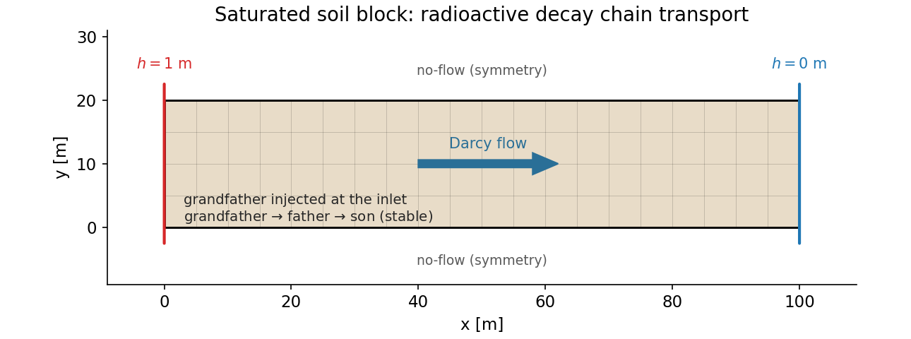
Figure 1: geometry, mesh and boundary conditions. Only the grandfather is injected; the father and son appear from decay along the flow path.

Geometry and boundary conditions

The soil block and flow BCs are those of the base case: \(h = 1\) m at the inlet (left, X0), \(h = 0\) m at the outlet (right, X1), no-flow top and bottom. At the inlet the grandfather is imposed at \(C = 1\) and the two daughters at \(C = 0\), so the profiles start from the Bateman initial condition (\(\tau = 0\)).

Numerical setup

Saturated single-phase CDO model, steady Richards equation, unsteady tracer equations. The chain is declared with cs_gwf_add_decay_chain (three species, mole units); each species gets the same transport parameters via cs_gwf_tracer_set_soil_param (no molecular diffusion, \(\alpha_L = 0.5\) m, no sorption). The run uses \(\Delta t = 10^5\) s for \(1200\) steps (\(1.2\times10^8\) s), long enough to reach steady state (about three domain transit times).

Running the simulation

cd CASE
code_saturne run --n 4

The mesh is generated internally. The run writes CASE/RESU/<id>/ with the hydraulic head and the three species grandfather, father and son in postprocessing/.

Results and verification

At steady state the three species partition along the flow path exactly as the Bateman solution predicts: the grandfather decays from the inlet, the father grows to a maximum near \(x \approx 39\) m and then decays, and the stable son accumulates monotonically. The computed molar fractions match the Bateman curves \(A(x/v)\), \(B(x/v)\), \(C(x/v)\) across the whole domain, and the three sum to one to better than \(10^{-6}\) (molar conservation of the chain).

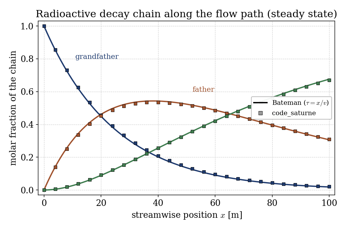
Figure 2: chain profiles at steady state (symbols) versus the Bateman solution mapped through $\tau = x/v$ (lines). The father ingrowth peak and the son accumulation are both recovered.

The only visible departure is a slight excess of the parent downstream, the expected footprint of the finite dispersion (the mapping \(\tau = x/v\) is exact only in the zero-dispersion limit).

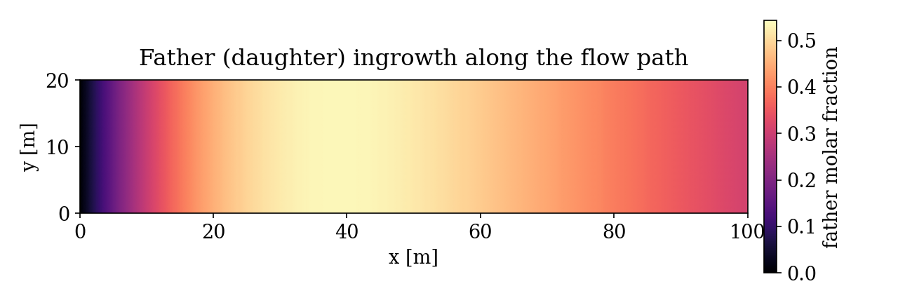
Figure 3: father (daughter) field. It is absent at the inlet, grows to a maximum where the grandfather has partly decayed, then fades as it decays into the son.

Summary

This tutorial carried a three-member radioactive decay chain through the saturated Darcy flow of the base case. Only the parent is injected; the intermediate and the stable end member appear from decay, giving the classic ingrowth picture. Because the transport is advection dominated, the steady-state spatial profiles reproduce the Bateman time solution through \(\tau = x/v\), and the chain conserves moles to round-off. The lesson that carries beyond this case: a decay chain is a set of tracer equations coupled by reaction source terms, set up in cs_user_parameters.cpp with a single cs_gwf_add_decay_chain call, and the groundwater module transports and reacts them together.

References

• H. Bateman. The solution of a system of differential equations occurring in the theory of radioactive transformations, Proc. Cambridge Philos. Soc. 15, 423-427, 1910.
• M. Th. van Genuchten. Convective-dispersive transport of solutes involved in sequential first-order decay reactions, Computers & Geosciences 11, 129-147, 1985.
• code_saturne documentation

Authors

Simvia. Questions, remarks and requests are welcome.