2D Mixer Vessel (Transient Rotor / Sliding Mesh)¶

Browse this case on GitHub

A step-by-step tutorial for simulating a baffled stirred tank with the transient rotor (sliding mesh) turbomachinery model of code_saturne: a four-blade impeller rotating at 60 rpm inside a cylindrical vessel equipped with four baffles. The companion tutorial Tbm_Mixer_Vessel_2D computes a similar configuration with the frozen rotor approximation on a single mesh; this one resolves the actual rotation: the rotor mesh turns rigidly at every time step, and the rotor/stator interface is re-joined on the fly.

Maintained by Simvia, part of the tutoriel-code_saturne collection.

Learning objectives¶

After completing this tutorial you will be able to:

Enable the transient rotor turbomachinery model (true sliding mesh).
Assemble a computation from two independent meshes (rotor + stator) connected by a face joining recomputed at every time step.
Choose a time step compatible with the sliding interface (fraction of a cell swept per step).
Post-process a rotating-mesh transient (probes in the fixed frame, EnSight output with transient connectivity).

Prerequisites¶

Requirement	Detail
code_saturne	v9.1
Case	Tbm_Mixer_Vessel_2D (frozen rotor companion case)

If code_saturne is not yet installed, build it from the official homepage, pull a ready-to-use Singularity image from the Open Simulation Center, or pull the Simvia Docker image before continuing.

Case files¶

Tbm_Mixer_Vessel_2D_Transient/
├── CASE/
│   └── DATA/
│       └── setup.xml            # pre-configured GUI case
├── MESH/
│   ├── rotor.msh                # rotating annulus, blades meshed as slits (gmsh, msh 4.1)
│   └── stator.msh               # fixed annulus, baffles meshed as slits (gmsh, msh 4.1)
├── FIGURES/                     # figures used in this README
└── README.md

Physical model¶

The flow is incompressible and laminar: at 60 rpm ($N = 1$ rev/s) the impeller Reynolds number, built on the impeller diameter $D = 0.095$ m, is

\[ Re = \frac{N D^2}{\nu} = \frac{1 \times 0.095^2}{10^{-5}} \approx 900 \]

so no turbulence model is used (contrast with the frozen rotor case at 1000 rpm, $Re \approx 1.7 \times 10^4$).

The transient rotor model is the reference approach for rotor/stator interaction: the cells of the rotor zone (and their walls) physically rotate at each time step, and the interface between the rotating and fixed parts of the mesh is a sliding, non-conforming joining whose connectivity is recomputed at every iteration. Unlike the frozen rotor model, it captures the true blade/baffle relative motion, at the price of a time-accurate (and therefore more expensive) computation.

Flow parameters¶

Quantity	Symbol	Value	Source in `setup.xml`
Density	$\rho$	$1\ \mathrm{kg\,m^{-3}}$	`density`
Molecular viscosity	$\mu$	$10^{-5}\ \mathrm{Pa\,s}$	`molecular_viscosity`
Rotation rate	$\omega$	$6.2832\ \mathrm{rad\,s^{-1}}$ (60 rpm)	`turbomachinery/rotor/velocity`
Blade tip speed	$\omega\, r_{tip}$	$0.298\ \mathrm{m\,s^{-1}}$	derived ($r_{tip} = 0.0475$ m)
Impeller Reynolds number	$Re$	$\approx 900$ (laminar)	derived

Geometry and meshes¶

The vessel is the same annular, quasi-2D layout as the frozen rotor case (outer radius $0.1$ m, hub radius $0.02$ m, one cell over a thickness of $0.01$ m), but the domain is now split into two independent gmsh meshes that meet at the interface radius $r = 0.06$ m:

Mesh	Extent	Cells	Obstacles
`rotor.msh`	$0.02 \le r \le 0.06$	$96 \times 16 = 1536$ hexahedra	4 blades at $0°/90°/180°/270°$, $0.02 < r < 0.0475$
`stator.msh`	$0.06 \le r \le 0.10$	$96 \times 16 = 1536$ hexahedra	4 baffles at $45°/135°/225°/315°$, $0.0725 < r < 0.10$

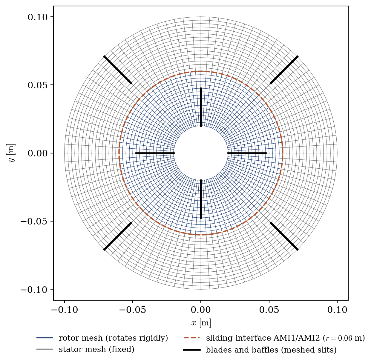
The two meshes: rotating rotor mesh (blue) and fixed stator mesh (gray), meeting at the dashed sliding interface, with blades and baffles meshed as slits.
Figure 1: the two-mesh assembly. The rotor mesh (blue) rotates rigidly; the stator mesh (gray) is fixed; they meet at the sliding interface (dashed circle, $r = 0.06$ m), carried by the boundary groups AMI1 (rotor side) and AMI2 (stator side). Blades and baffles are meshed as zero-thickness slits (duplicated nodes), so no thin-wall insertion is needed here, unlike in the frozen rotor case.

The sliding interface¶

Each mesh is a closed annulus: the outer boundary of rotor.msh (group AMI1) and the inner boundary of stator.msh (group AMI2) are two coincident rings of 96 boundary faces each. Without further action they would be two watertight default walls. The face_joining defined inside the turbomachinery section (selector AMI1 or AMI2) glues them into interior faces; being attached to the transient rotor model, this joining is recomputed at every time step, after the rotor mesh has rotated: this is the sliding-mesh mechanism, and the joined faces are generally non-conforming.

Rotor zone and boundary conditions¶

Only the rotating part is declared: the rotor zone is selected by the volume group rotor_fluid of rotor.msh, and everything else is stator (fixed) by default. The walls carried by rotor cells (hub and blades) automatically rotate with the zone.

Boundary	Location	Nature	Zone selector
`rotor_wall`	hub + blades	Smooth wall (rotating)	`rotor`
`stator_wall`	tank wall + baffles	Smooth wall	`stator`
`front`, `back`	spanwise planes	Symmetry	`front`, `back`

Note on gmsh formats: these meshes are in msh 4.1 format, for which code_saturne attaches the physical names to the groups (selectors like rotor, AMI1 or rotor_fluid work directly). This differs from the older msh 2.2 format used in the frozen rotor case, where only the numeric physical tags are available.

Numerical setup¶

Setting	Value	Rationale
Turbomachinery model	Transient rotor	True sliding mesh
Rotor zone	`rotor_fluid`	The whole rotor mesh rotates
Interface	`face_joining` on `AMI1 or AMI2`	Re-joined at every time step
Velocity-pressure coupling	SIMPLEC	Standard segregated coupling
Time-stepping	Fixed $\Delta t = 10^{-3}$ s	$0.36°$ of rotation per step, about $1/10$ of an azimuthal cell at the interface
Simulated time	$5$ s ($5000$ steps, 5 revolutions)	Rotating-core flow established; see the spin-up caveat below
Turbulence	none (laminar)	$Re \approx 900$
Output	EnSight every $100$ steps, transient connectivity	The mesh moves: the geometry is rewritten at each output
Probes	4, recorded every step	All in the fixed stator region

Running the simulation¶

The commands below start from the tutorial directory:

cd Tbm_Mixer_Vessel_2D_Transient/

Option A: Graphical interface¶

code_saturne gui CASE/DATA/setup.xml &

The GUI opens the pre-configured setup.xml. Review the setup if you wish, then launch the run with the gear (Run) button in the toolbar.

Option B: Command line¶

The command-line launcher is run from inside the case directory:

cd CASE

# serial
code_saturne run

# parallel (e.g. 2 MPI ranks)
code_saturne run --n 2

Each run creates a time-stamped directory CASE/RESU/<YYYYMMDD-HHMM>/ containing:

run_solver.log: solver log (look for the unsteady rotor/stator treatment summary and the joining information at each step),
monitoring/probes_*.csv: probe histories,
postprocessing/: time series of volume fields in EnSight Gold format, with one geometry per output time.

Results¶

The rotor really rotates¶

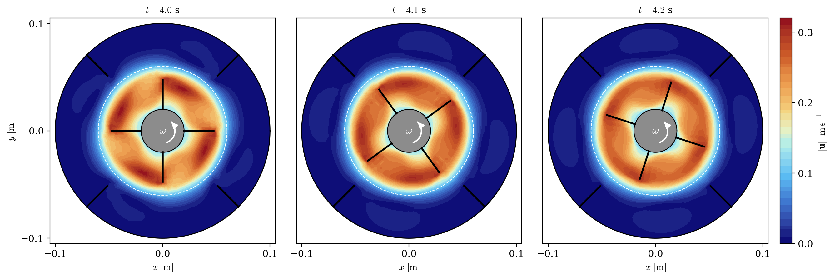
Velocity magnitude at t = 4.0, 4.1 and 4.2 s: the blades advance by 36 degrees between snapshots while the baffles stay fixed.
Figure 2: Velocity magnitude at $t = 4.0$, $4.1$ and $4.2$ s (the white arrow marks the rotation direction). Between two snapshots the impeller advances by $36°$ while the baffles stay fixed: the blade/baffle relative position, frozen by assumption in the companion case, is resolved here. The high-velocity lobes trail the blades, and the baffled outer region stays quiet.

Spin-up and probes¶

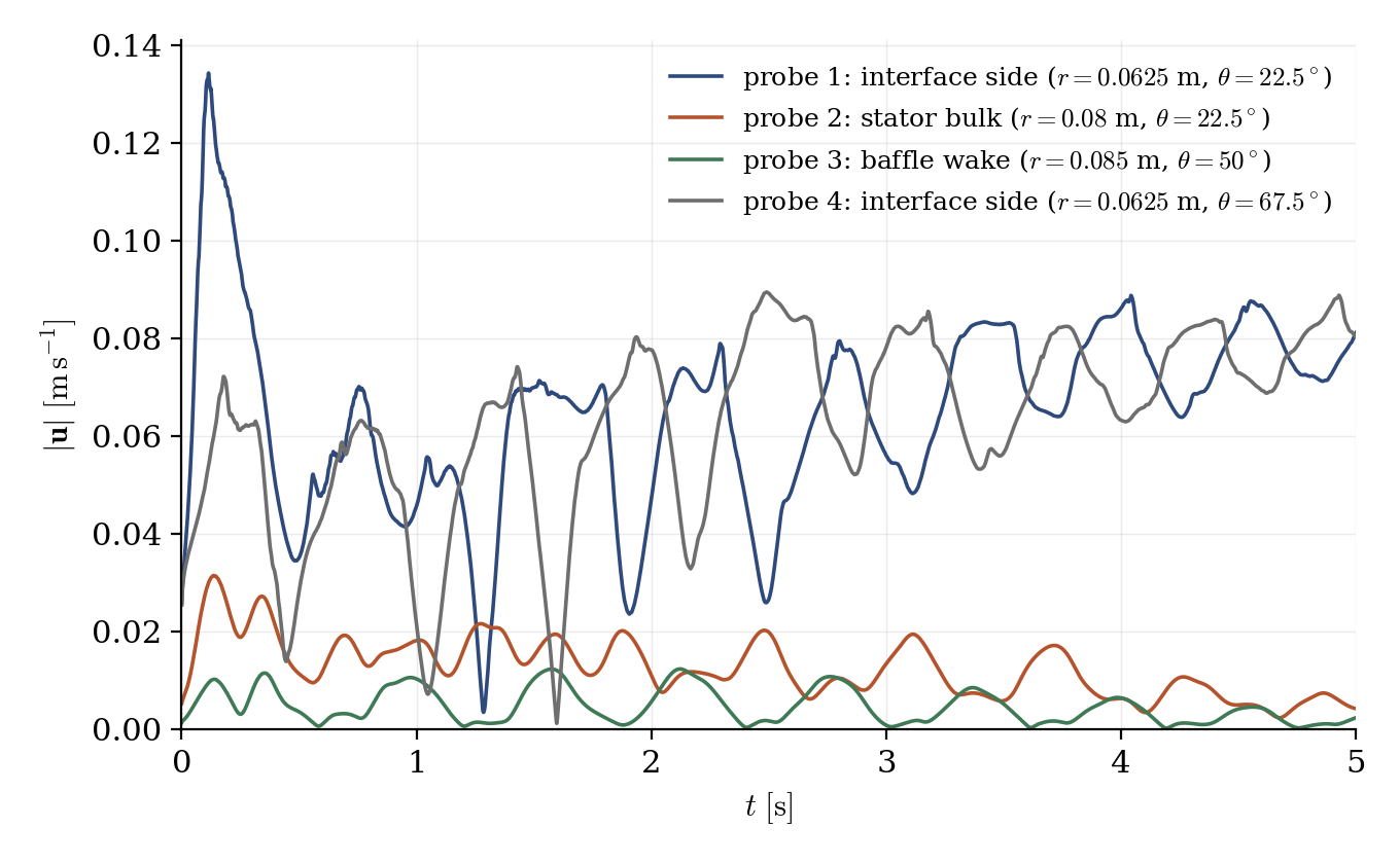
Velocity magnitude histories at the four monitoring probes over the five revolutions.
Figure 3: Velocity magnitude at the four monitoring probes (all in the fixed stator region). The near-interface probes (1 and 4) oscillate as the rotor structures sweep past them; the bulk and baffle-wake probes show the slow laminar spin-up of the outer region.

An honest caveat on convergence: at $Re \approx 900$ the flow spins up on the viscous time scale $\tau_\nu \sim \Delta r^2/\nu \sim 10^2$ s, so after 5 revolutions ($5$ s) only the rotor core is established; the stator bulk is still slowly accelerating, as probe 2 shows. This is the physics of laminar stirred tanks, not a numerical artifact; running the case longer simply continues the spin-up. The purpose of this tutorial is the sliding-mesh workflow, which is fully exercised here.

Summary¶

This tutorial computed a baffled stirred tank with the transient rotor (sliding mesh) model of code_saturne: two independent gmsh meshes glued by a face joining recomputed at every time step, a rotor zone selected by its volume group, blades and baffles meshed as zero-thickness slits, and a time step chosen so the interface slides by a fraction of a cell per step. Together with Tbm_Mixer_Vessel_2D (frozen rotor), it covers the two turbomachinery approaches of code_saturne.

References¶

code_saturne documentation
E.L. Paul, V.A. Atiemo-Obeng, S.M. Kresta (eds). Handbook of Industrial Mixing: Science and Practice, Wiley, 2004.

Authors¶

Simvia - Questions, remarks and requests are welcome.

Quantity	Symbol	Value	Source in `setup.xml`
Density	\(\rho\)	\(1\ \mathrm{kg\,m^{-3}}\)	`density`
Molecular viscosity	\(\mu\)	\(10^{-5}\ \mathrm{Pa\,s}\)	`molecular_viscosity`
Rotation rate	\(\omega\)	\(6.2832\ \mathrm{rad\,s^{-1}}\) (60 rpm)	`turbomachinery/rotor/velocity`
Blade tip speed	\(\omega\, r_{tip}\)	\(0.298\ \mathrm{m\,s^{-1}}\)	derived (\(r_{tip} = 0.0475\) m)
Impeller Reynolds number	\(Re\)	\(\approx 900\) (laminar)	derived

Mesh	Extent	Cells	Obstacles
`rotor.msh`	\(0.02 \le r \le 0.06\)	\(96 \times 16 = 1536\) hexahedra	4 blades at \(0°/90°/180°/270°\), \(0.02 < r < 0.0475\)
`stator.msh`	\(0.06 \le r \le 0.10\)	\(96 \times 16 = 1536\) hexahedra	4 baffles at \(45°/135°/225°/315°\), \(0.0725 < r < 0.10\)