Rayleigh-Taylor Instability (VOF)
A step-by-step tutorial for simulating the Rayleigh-Taylor instability with the VOF (Volume of Fluid) model of code_saturne: a heavy fluid rests on top of a light fluid under gravity, and any perturbation of the interface grows into the characteristic falling spikes and rising bubbles. Together with Vof_Kelvin_Helmholtz, it is a compact demonstration of a two-phase VOF setup.
Maintained by Simvia, part of the tutoriel-code_saturne collection.
Learning objectives
After completing this tutorial you will be able to:
- Set up a gravity-driven two-phase problem with the VOF homogeneous model.
- Initialize the void fraction with a
cs_user_initialization.cppuser routine (the velocity stays at rest: the instability is driven by gravity alone). - Use a CFL-controlled adaptive time step for a flow whose velocities grow in time.
- Run the case and visualize the void fraction field (spikes, bubbles, mushrooms).
Prerequisites
| Requirement | Detail |
|---|---|
| code_saturne | v9.1 |
| Case | Vof_Kelvin_Helmholtz (details of the VOF model) |
If code_saturne is not yet installed, build it from the official homepage, pull a ready-to-use Singularity image from the Open Simulation Center, or pull the Simvia Docker image before continuing.
Case files
Vof_Rayleigh_Taylor/
├── CASE/
│   ├── DATA/
│   │   └── setup.xml                    # pre-configured GUI case
│   └── SRC/
│       └── cs_user_initialization.cpp   # sinusoidally perturbed interface
├── FIGURES/                             # figures used in this README
└── README.md
There is no MESH directory: the mesh is generated at run time by the built-in cartesian mesher (\(64 \times 192 \times 1\) cells on \([0,1] \times [-1, 2]\)).
Physical model
The VOF homogeneous model solves the incompressible momentum equations for the mixture plus one transport equation for the void fraction \(\alpha\), from which the mixture density and viscosity follow algebraically; the interface is implicit (see the Vof_Kelvin_Helmholtz tutorial for the equations).
Here the heavy phase (\(\alpha = 1\), \(\rho_1 = 5\)) rests on top of the light phase (\(\alpha = 0\), \(\rho_0 = 1\)) under a downward gravity \(g = 1\ \mathrm{m\,s^{-2}}\): the configuration is unstable, with an Atwood number
The initial state, set by cs_user_initialization.cpp, is a fluid at rest with a sinusoidally displaced interface (single mode \(k = 2\pi\), one wavelength in the periodic box):
The perturbation grows under gravity: the heavy fluid sinks as a spike, the light fluid rises as bubbles, and the shear along the spike flanks triggers secondary Kelvin-Helmholtz roll-ups, producing the classical mushroom shapes.
Flow parameters
| Quantity | Symbol | Value | Source in setup.xml / SRC |
|---|---|---|---|
| Phase densities | \(\rho_0\), \(\rho_1\) | \(1.0\), \(5.0\) | density (per-phase values) |
| Atwood number | \(A\) | \(0.667\) | derived |
| Phase viscosities | \(\mu_0\), \(\mu_1\) | \(10^{-3}\), \(10^{-3}\) | molecular_viscosity |
| Gravity | \(g\) | \((0, -1, 0)\ \mathrm{m\,s^{-2}}\) | gravity |
| Surface tension | \(\sigma_s\) | \(0\) | surface_tension |
| Interface position, amplitude | \(y_0\), \(\varepsilon\) | \(1.0\), \(0.03\) m | cs_user_initialization.cpp |
| Seeded mode | \(k\) | \(2\pi\) | cs_user_initialization.cpp |
| Domain | \([0,1] \times [-1,2]\), \(64 \times 192\) cells | mesh_cartesian |
|
| Time step | \(\Delta t\) | adaptive, CFL \(\le 1\) (seed \(5 \times 10^{-4}\) s) | time_parameters |
| Final time | \(t_{end}\) | \(4.4\) s | maximum_time |
Geometry and boundary conditions
The domain is a tall box, periodic in \(x\), with symmetry planes at the top and bottom. The interface starts at \(y_0 = 1\), which leaves two meters of fall for the heavy spike below and one meter above for the rising bubbles. The two spanwise (\(xy\)) planes carry a symmetry condition, so the computation is effectively two-dimensional.
| Boundary | Location | Nature | Zone |
|---|---|---|---|
| periodic pair | \(x = 0\) and \(x = 1\) | Periodicity (translation) | X0, X1 |
Y0, Y1 |
\(y = -1\), \(y = 2\) | Symmetry | Y0, Y1 |
Z0, Z1 |
spanwise planes | Symmetry | Z0, Z1 |
The initial state is set by SRC/cs_user_initialization.cpp, compiled automatically at the beginning of the run (the routine does not overwrite the fields on a restart).
Numerical setup
| Setting | Value | Rationale |
|---|---|---|
| Velocity-pressure coupling | SIMPLEC | Standard segregated coupling |
| Two-phase model | VOF, no mass transfer | Single \(\alpha\) transport equation, implicit interface |
| Time-stepping | Adaptive, max CFL \(= 1\) | The fall velocity grows in time: the step adapts (contrast with the fixed step of the Kelvin-Helmholtz case) |
| Turbulence | none (laminar) | Laminar two-phase demonstration |
| Output frequency | every 10 time steps | Time series of the void fraction |
Running the simulation
The commands below start from the tutorial directory:
cd Vof_Rayleigh_Taylor/
Option A: Graphical interface
code_saturne gui CASE/DATA/setup.xml &
The GUI opens the pre-configured setup.xml. Review the setup if you wish,
then launch the run with the gear (Run) button in the toolbar.
Option B: Command line
The command-line launcher is run from inside the case directory:
cd CASE

# serial
code_saturne run

# parallel (e.g. 2 MPI ranks)
code_saturne run --n 2
The user routine SRC/cs_user_initialization.cpp is compiled automatically at the beginning of the run.
Each run creates a time-stamped directory CASE/RESU/<YYYYMMDD-HHMM>/ containing:
run_solver.log: solver log,postprocessing/: time series of volume fields in EnSight Gold format.
Results
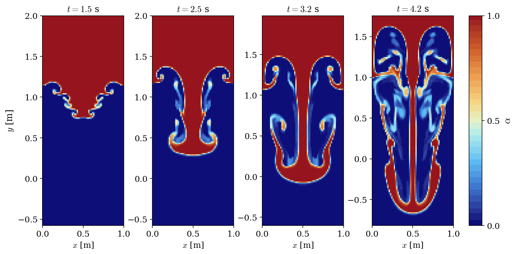
Figure 1: Void fraction $\alpha$ at $t = 1.5$, $2.5$, $3.2$ and $4.2$ s: the perturbed interface steepens, the heavy spike falls while the light bubbles rise, secondary Kelvin-Helmholtz roll-ups develop on the spike flanks, and the flow evolves into the classical mushroom structures. The fields are shifted along the periodic $x$ direction to center the spike, and the vertical window of each panel follows the falling structure (same window height on all panels).
Summary
This tutorial set up a Rayleigh-Taylor instability with the VOF model of code_saturne: heavy fluid over light fluid under gravity, void fraction initialized by a user routine with the flow at rest, streamwise periodicity, and a CFL-controlled adaptive time step. The interface evolves into the classical spikes, bubbles and mushrooms, with secondary Kelvin-Helmholtz roll-ups along the spike. Together with Vof_Kelvin_Helmholtz, it covers the two canonical interfacial instabilities with the VOF model.
References
- Lord Rayleigh. Investigation of the character of the equilibrium of an incompressible heavy fluid of variable density, Proc. London Math. Soc., 14:170-177, 1883.
- G.I. Taylor. The instability of liquid surfaces when accelerated in a direction perpendicular to their planes, Proc. R. Soc. Lond. A, 201:192-196, 1950.
- code_saturne documentation
Authors
Simvia - Questions, remarks and requests are welcome.