Boundary-Layer Insertion (Prism Layers at the Walls)¶

Browse this case on GitHub

A step-by-step tutorial for the boundary-layer insertion operation of code_saturne: starting from a mesh with no near-wall refinement, cs_mesh_boundary_layer_insert deflates the interior mesh away from selected walls and fills the freed space with layers of prisms, at run time. This is the rescue tool for meshes that arrive without boundary layers (imported geometries, quick cartesian blocks). Two cases are shipped, identical but for one file: the 25-line user routine that inserts the layers.

Unlike face joining or extrusion, this operation has no GUI page in this version: it lives in cs_user_mesh.cpp (the cs_user_mesh_modify function). Everything else in the case remains GUI-configured.

Maintained by Simvia, part of the tutoriel-code_saturne collection.

Learning objectives¶

After completing this tutorial you will be able to:

Insert prism layers on selected walls from cs_user_mesh_modify (the extrude_face_info → extrude_vectors → boundary_layer_insert API trio).
Choose the layer parameters (number, total thickness, expansion factor) and avoid the sign trap of the expansion semantics.
Check the operation: insertion report in the log, mesh inspection, near-wall cell size before/after.

Prerequisites¶

Requirement	Detail
code_saturne	v9.1
Tutorial	Pre_Face_Joining (the 05_preprocessing workflow: preprocessing runs, reading the mesh reports)

If code_saturne is not yet installed, build it from the official homepage, pull a ready-to-use Singularity image from the Open Simulation Center, or pull the Simvia Docker image before continuing.

Case files¶

Pre_Boundary_Layer/
├── CASE_Uniform/
│   └── DATA/setup.xml        # coarse uniform mesh, no SRC
├── CASE_Layers/
│   ├── DATA/setup.xml        # identical
│   └── SRC/cs_user_mesh.cpp  # THE difference: 4 layers on the walls
├── FIGURES/                  # figures used in this README
└── README.md

The mesh is generated by the built-in cartesian mesher; the two setup.xml are identical (only the case name differs). The whole operation is the one routine.

The case¶

The support flow is deliberately unremarkable: a turbulent air channel ($0.1 \times 2$ m, $10$ m/s, $k$-$\varepsilon$ with wall functions) on a coarse $100 \times 10$ cartesian mesh: $10$ uniform cells across the height, so a wall-adjacent cell of $10$ mm. The routine inserts, on both walls:

4 layers over a total thickness of 15 mm with an expansion factor of 0.7;
the wall selection reuses the same criteria string as the boundary condition (Y0 or Y1).

One semantic trap is worth the detour: the expansion factor is the ratio between successive layers along the insertion direction, which runs from the deflated interior surface toward the wall. A factor below one therefore puts the thinnest layer against the wall ($\approx 2$ mm here); a factor above one would put it against the interior, the opposite of a boundary layer.

Sizing the layers¶

The layer widths form a geometric sequence: first width $a$ on the interior side, then $ar, ar^2, \dots, ar^{\,n-1}$ down to the wall. The two useful relations, with $e_{tot}$ the total thickness (the API argument) and $e_{wall}$ the wall-adjacent width (what you are after):

\[ e_{tot} = a\,\frac{1 - r^{\,n}}{1 - r}, \qquad e_{wall} = a\,r^{\,n-1} \]

In practice you know the interior cell size $h$ and the wall width $e_{wall}$ you want; taking $a \approx h$ for size continuity at the layer/interior junction, choose the number of layers $n$ and the two API parameters follow:

\[ r = \Big(\frac{e_{wall}}{h}\Big)^{\frac{1}{n-1}}, \qquad e_{tot} = h\,\frac{1 - r^{\,n}}{1 - r} \]

Here: $h \approx 7$ mm (the 10 interior cells share the height minus the two inserted thicknesses), target $e_{wall} = 2$ mm, $n = 4$ → $r = (2/7)^{1/3} \approx 0.7$ and $e_{tot} \approx 15$ mm, the values in the routine. Note that $h$ itself shrinks a little when the layers take their room (the deflation), so one quick iteration of these formulas is enough to converge the design.

Two safeguards are worth knowing: the min_volume_factor argument (here $0.2$) limits how much the deflation may squeeze any interior cell, and the deflation displacement is solved as a CDO mesh-deformation problem at startup (a few extra lines in the log, negligible cost).

Running the simulation¶

The commands below start from the tutorial directory:

cd Pre_Boundary_Layer/

Run both cases (GUI: open each setup.xml and use the Run button; the routine in SRC/ is compiled automatically):

cd CASE_Uniform
code_saturne run --id uniform

cd ../CASE_Layers
code_saturne run --id layers

In the CASE_Layers log, the insertion reports itself during mesh preparation:

Extrusion: 200 boundary faces selected.
           800 cells added.

and the mesh summary goes from $1000$ cells (CASE_Uniform) to $1800$. A mesh-preprocessing-only run (code_saturne run --initialize) is the natural first step here too, to inspect the modified mesh before computing.

Results¶

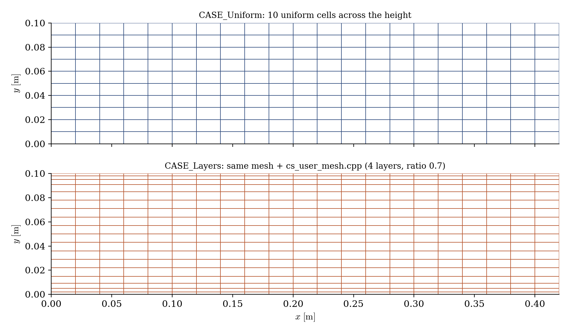
The same channel mesh before and after insertion: four prism layers hug each wall, the interior cells are pushed inward.
Figure 1: the mesh near the inlet, before (top) and after (bottom) the insertion. The interior mesh is deflated away from the walls and four layers of thickness ratio $0.7$ fill the freed $15$ mm, the thinnest ($\approx 2$ mm) against each wall.

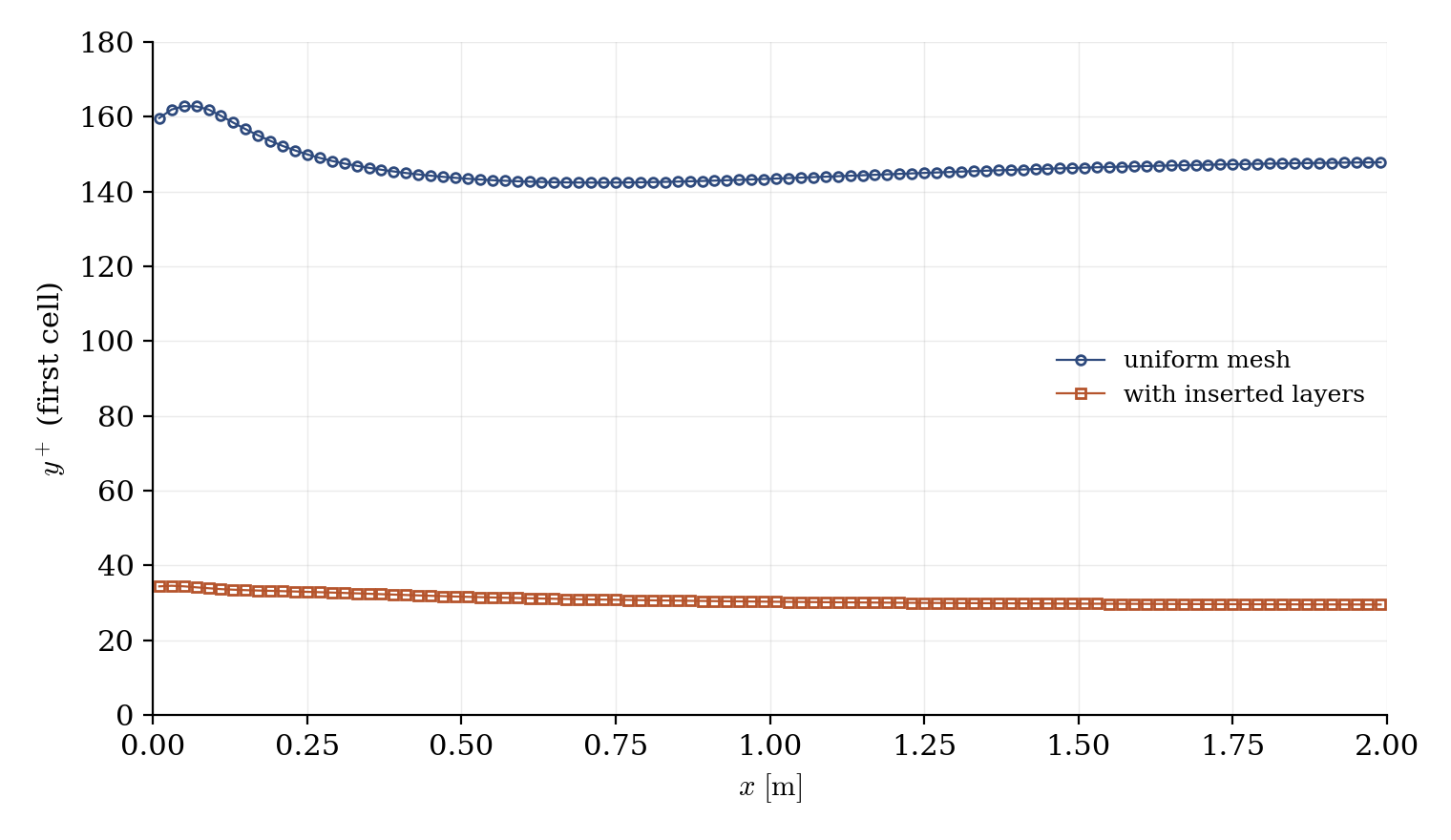
First-cell y+ along the wall, about five times smaller with the inserted layers.
Figure 2: the practical effect, read through the standard indicator of near-wall resolution: the first-cell $y^+$ drops from $\approx 146$ to $\approx 30$, i.e. into the range wall functions are designed for.

Summary¶

This tutorial inserted prism layers on the walls of an existing mesh with cs_mesh_boundary_layer_insert, driven by a 25-line cs_user_mesh_modify routine, the only difference between the two shipped cases (this operation has no GUI page in this version). Key facts to remember: the wall selection is an ordinary criteria string, the expansion factor must be below one for the thinnest layer to land against the wall, and the log reports the operation (800 cells added). The near-wall cell size drops by a factor of five, as Figure 2 shows on the $y^+$ indicator.

References¶

code_saturne documentation

Authors¶

Simvia - Questions, remarks and requests are welcome.