Porous Plug in a Duct

Browse this case on GitHub

A step-by-step tutorial for using a porosity zone in code_saturne: a volume region where only a fraction \(\varepsilon\) of the space is open to the flow, as in a packed bed, a tube bundle or a debris screen. A uniform stream crosses a 0.2 m plug of porosity \(\varepsilon = 0.5\), and the velocity inside doubles, exactly as mass conservation dictates. The case is the mirror of Inc_Head_Loss_Zone: porosity rescales the flow geometry seen by all the conservation equations without adding any source term, whereas a head loss adds an explicit friction source term to the momentum equation; a real porous medium generally needs both. The whole setup is done in the GUI: no mesh file, no user routine.

Maintained by Simvia, part of the tutoriel-code_saturne collection.

Learning objectives

After completing this tutorial you will be able to:

1. Define a porosity zone with a geometric criterion and a MEG formula.
2. Know which velocity code_saturne resolves in a porous region (the interstitial one), and verify it with mass conservation.
3. Tell apart the roles of porosity and head losses, and know when each (or both) is needed.

Prerequisites

Requirement	Detail
code_saturne	v9.1
Case	Inc_Head_Loss_Zone (the momentum half of the story)

If code_saturne is not yet installed, build it from the official homepage, pull a ready-to-use Singularity image from the Open Simulation Center, or pull the Simvia Docker image before continuing.

Case files

Inc_Porous_Plug/
├── CASE/
│   └── DATA/
│       └── setup.xml            # pre-configured GUI case
├── FIGURES/                     # figures used in this README
└── README.md

There is no MESH directory (built-in cartesian mesher) and no SRC directory: everything is set in the GUI.

Physical model

In a porosity zone, only the fraction \(\varepsilon\) of each cell (and of each face) is open to the flow. code_saturne resolves the interstitial velocity \(\mathbf{u}\) (the velocity of the fluid where it actually flows), and weights the fluxes by the porosity: mass conservation through a constant-section duct then reads

\[ \varepsilon\, u = U = \mathrm{const} \]

so the flow accelerates inside the plug: with \(\varepsilon = 0.5\) and \(U = 1\ \mathrm{m\,s^{-1}}\), the interstitial velocity is \(u = 2\ \mathrm{m\,s^{-1}}\). The porosity weights the momentum equation as well (fluid volumes, convective fluxes): the model adds no friction term anywhere, but the flow still pays singular head losses at the two ends of the plug, where it sees a sudden contraction (entry) and a sudden expansion (exit), exactly as it would at abrupt section changes of a duct.

To represent a real porous medium (a packed bed, a filter cake), the porosity must be combined with a head-loss zone carrying the Darcy-Forchheimer resistance of the matrix: porosity for the kinematics, head loss for the friction. That combination, calibrated with the Ergun correlation, is the object of a follow-up case.

Flow parameters

Quantity	Symbol	Value	Source in setup.xml
Fluid (air-like)	\(\rho\), \(\mu\)	\(1.2\ \mathrm{kg\,m^{-3}}\), \(1.8 \times 10^{-5}\ \mathrm{Pa\,s}\)	density, molecular_viscosity
Inlet velocity	\(U\)	\(1\ \mathrm{m\,s^{-1}}\)	inlet/velocity_pressure/norm
Plug porosity	\(\varepsilon\)	\(0.5\)	porosities/porosity (MEG formula)
Plug thickness	\(L\)	\(0.2\) m (\(x = 0.4\) to \(0.6\))	zone selector
Expected in-plug velocity	\(U/\varepsilon\)	\(2\ \mathrm{m\,s^{-1}}\)	derived
Domain, mesh		\(1 \times 0.1 \times 0.02\) m, \(200 \times 20 \times 1\) cells	mesh_cartesian
Time	\(\Delta t\), \(N\)	\(2 \times 10^{-3}\) s, \(1000\) steps	time_parameters

Geometry and boundary conditions

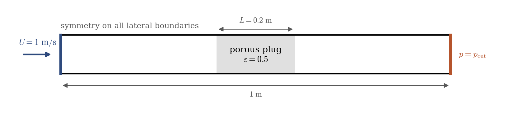
Figure 1: computational domain, identical to the head-loss case except for the nature of the zone. All lateral boundaries are symmetries: the stream is a uniform plug flow and the profiles below are one-dimensional.

Boundary	Location	Nature	Zone selector
Inlet	\(x = 0\)	Velocity inlet, \(1\ \mathrm{m\,s^{-1}}\)	X0
Outlet	\(x = 1\)	Free outlet	X1
SymY, SymZ	lateral faces	Symmetry	Y0 or Y1, Z0 or Z1

The porosity zone in the GUI

Two steps, exactly parallel to the head-loss workflow:

1. Volume zones: add a zone (here porous_plug) with the selection criterion box[0.4, -0.01, -0.01, 0.6, 0.11, 0.03] and tick the Porosity nature.
2. Volume conditions → Porosity: select the zone, the isotropic model, and enter the MEG formula porosity = 0.5; (a formula rather than a constant: the porosity may vary in space).

Numerical setup

Setting	Value	Rationale
Velocity-pressure coupling	SIMPLEC	Standard segregated coupling
Velocity convection scheme	1st-order upwind (blending_factor 0)	The centered scheme sustains a small standing wave trapped between the two porosity jumps (a limit cycle at the plug transit period); upwind damps it, at no cost on a piecewise-constant solution
Time-stepping	Fixed \(\Delta t = 2 \times 10^{-3}\) s, \(1000\) steps	In-plug CFL \(< 1\) (the velocity doubles there), 2 flow-through times
Turbulence	none (laminar)	Plug flow with slip boundaries
Initialization	\(u = U\) everywhere	Converges in a handful of iterations
Probes	6 along the axis	2 upstream, 2 inside the plug, 2 downstream

Running the simulation

The commands below start from the tutorial directory:

cd Inc_Porous_Plug/

Option A: Graphical interface

code_saturne gui CASE/DATA/setup.xml &

The GUI opens the pre-configured setup.xml. Review the setup if you wish, then launch the run with the gear (Run) button in the toolbar.

Option B: Command line

The command-line launcher is run from inside the case directory:

cd CASE

# serial (a few seconds)
code_saturne run

Results

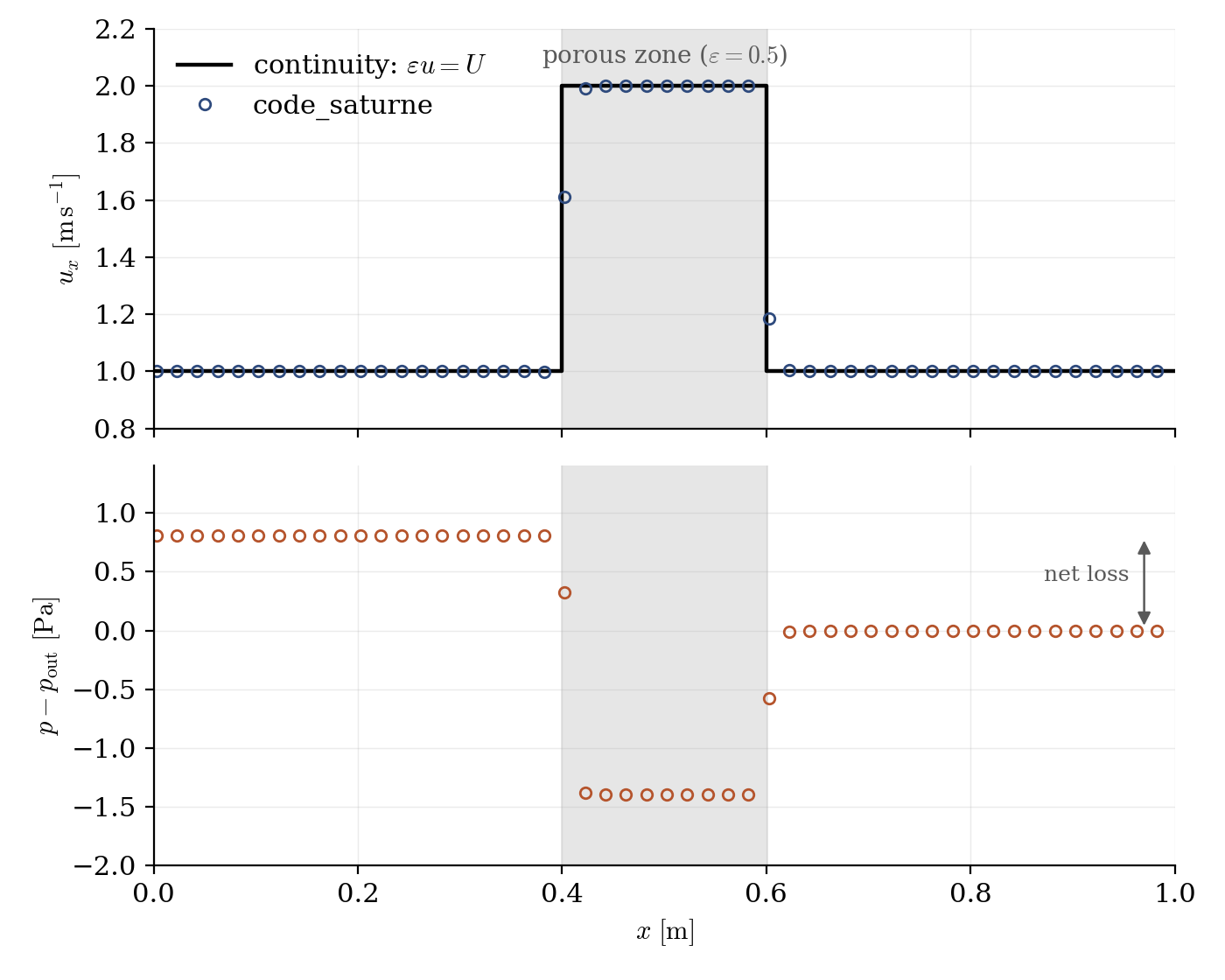
Figure 2: velocity (top) and pressure (bottom) along the duct at steady state. The interstitial velocity inside the plug is $2.000\ \mathrm{m\,s^{-1}}$, matching $\varepsilon u = U$ exactly (the transition spans the one or two cells over which the porosity jumps). The pressure drops where the flow accelerates into the plug and recovers only partially at the exit: the difference between the two plateaus is the sum of the singular losses of the sudden contraction (entry) and the sudden expansion (exit).

The net loss between the two plateaus (\(0.81\) Pa) is the signature of these two singular losses. Its exact value should not be over-interpreted: the section change is not resolved (the porosity jumps across a single mesh face), and for a real porous medium these end effects are lumped into the bed correlations anyway.

Note that the pressure is flat inside the plug : the porosity model exerts no distributed friction, only the singular entry/exit effects of the section change. For a real packed bed this is the wrong balance by orders of magnitude: with \(1\) mm spheres at \(\varepsilon = 0.5\) under the same flow, the Ergun correlation gives an internal gradient of \(\approx 14\,\mathrm{kPa/m}\), i.e. \(\approx 2800\) Pa across these \(0.2\) m, against the \(0.8\) Pa of entry/exit losses computed here. That distributed friction is exactly what a head-loss zone carries, hence the follow-up case combining both.

Contrast with Inc_Head_Loss_Zone: there, the velocity stayed uniform and the zone created a prescribed pressure drop; here, the velocity jumps and the pressure change is a consequence of the kinematics alone. The two features answer two different questions, and a real porous medium needs both.

Summary

This tutorial set up a porosity zone in a duct: a volume zone selected by a geometric criterion, the porosity given by a MEG formula, and the computed interstitial velocity equal to \(U/\varepsilon\) exactly, as mass conservation requires. Together with the head-loss case it clarifies the division of labor: porosity changes the geometry seen by all the equations (interstitial acceleration and singular entry/exit effects follow from conservation, with no added term), head losses add the explicit distributed friction of the matrix; combining them, with coefficients from the Ergun correlation, models a real packed bed.

References

• I.E. Idelchik. Handbook of Hydraulic Resistance, 4th edition, Begell House, 2007.
• S. Ergun. Fluid flow through packed columns, Chem. Eng. Prog., 48:89-94, 1952.
• code_saturne documentation

Authors

Simvia - Questions, remarks and requests are welcome.