Laval Nozzle with a Normal Shock

Browse this case on GitHub

This tutorial computes one operating point with the compressible module of code_saturne: a choked nozzle with a normal shock standing in the divergent. A single run therefore contains a subsonic acceleration, a sonic throat, a supersonic expansion, a shock, and a subsonic recompression to the imposed exit pressure, and every one of those is verified against the quasi-1D exact solution.

Maintained by Simvia, part of the tutoriel-code_saturne collection.

Learning objectives

After completing this tutorial you will be able to:

1. Set the operating point of a compressible internal flow with the pair of boundary conditions that decides it: total conditions (\(P_t\), \(H_t\)) at the inlet and an imposed static pressure at a subsonic outlet.
2. Build a shaped duct without any mesh file, by squeezing a Cartesian slab in cs_user_mesh_modify.
3. Verify a computation against the area-Mach relation, and locate a normal shock from the back pressure alone.

Prerequisites

Requirement	Detail
code_saturne	v9.1
Tutorials	Comp_Sod_Tube (compressible module, exact Euler limit), Comp_Supersonic_Ramp (shock capture)
Background	Gas dynamics: isentropic relations, normal shock relations

If code_saturne is not yet installed, build it from the official homepage, pull a ready-to-use Singularity image from the Open Simulation Center, or pull the Simvia Docker image before continuing.

Case files

Comp_Laval_Nozzle/
├── CASE/
│   ├── DATA/
│   │   └── setup.xml            # pre-configured GUI case
│   └── SRC/
│       └── cs_user_mesh.cpp     # the nozzle geometry: slab, then area law
├── FIGURES/                     # figures used in this README
└── README.md

There is no mesh file. The nozzle is a Cartesian slab whose height is squeezed by the area law, and that law is written once, in cs_user_mesh.cpp, which is also the function the verification below uses. There is no second copy of the geometry to keep in step with the first.

Physical model

The flow is steady, two-dimensional and inviscid: the Euler equations for a perfect gas with \(\gamma = 1.4\). The inviscid limit is enforced exactly by GUI user laws setting the molecular viscosity, the volume viscosity and the thermal conductivity to zero, as in Comp_Sod_Tube (a GUI constant cannot be zero, a user-law formula can).

What the theory predicts

For a slender duct the flow is nearly one-dimensional, and the isentropic relations tie the local Mach number to the local area alone:

\[ \frac{A}{A^*} = \frac{1}{M}\left[\frac{2}{\gamma+1} \left(1 + \frac{\gamma-1}{2}M^2\right)\right]^{\frac{\gamma+1}{2(\gamma-1)}} \]

where \(A^*\) is the sonic section. Once the throat is choked, \(A^* = A_t\) upstream of the shock, the mass flow is fixed at its critical value, and the back pressure can no longer influence the convergent at all.

A normal shock in the divergent does not change the mass flow, but it destroys total pressure, so the sonic section grows across it:

\[ \frac{A_2^*}{A_1^*} = \frac{p_{t1}}{p_{t2}} \]

Downstream of the shock the flow is subsonic again and follows the same area-Mach relation, now with \(A_2^*\). That chain closes the problem: the shock sits exactly where the resulting exit pressure matches the imposed one. Here, \(p_\mathrm{out}/p_0 = 0.679\) places it at \(x = 0.691\) m, with \(M_1 = 1.902\) just upstream and \(M_2 = 0.595\) just downstream.

Flow parameters

Quantity	Symbol	Value	Source in setup.xml
Heat capacity ratio	\(\gamma\)	\(1.4\)	from specific_heat (\(1004.85\)) and reference_molar_mass
Inlet total pressure	\(p_0\)	\(101\,325\) Pa	inlet/velocity_pressure/total_pressure
Inlet total enthalpy	\(H_t = c_p T_0\)	\(301\,455\) J/kg	inlet/velocity_pressure/enthalpy
Inlet total temperature	\(T_0\)	\(300\) K	(derived from \(H_t\))
Imposed exit pressure	\(p_\mathrm{out}\)	\(68\,845\) Pa	outlet/dirichlet name="pressure"
Pressure ratio	\(p_\mathrm{out}/p_0\)	\(0.679\)	(derived)
Viscosity, conductivity	\(\mu\), \(\lambda\)	\(0\) (exact Euler limit)	user laws in fluid_properties

Geometry and boundary conditions

The nozzle is 1 m long. Its half height follows a smoothstep on each side of the throat, which puts \(\mathrm{d}A/\mathrm{d}x = 0\) at the throat (a genuine sonic section) and at both ends (so the inlet and outlet planes are flat and the boundary conditions stay one-dimensional):

\[ h(x) = h_t + (h_e - h_t)\, s^2(3 - 2s), \qquad s = \frac{x - x_t}{L - x_t} \ \ \text{in the divergent} \]

Station	\(x\) [m]	Half height [m]	\(A/A_t\)
Inlet	\(0.00\)	\(0.100\)	\(2\)
Throat	\(0.35\)	\(0.050\)	\(1\)
Outlet	\(1.00\)	\(0.100\)	\(2\)

The maximum wall slope of the divergent is 6.6 degrees. That number is a design constraint, not a detail: quasi-1D theory assumes the flow stays nearly axial, so the nozzle has to be slender for the comparison below to mean anything.

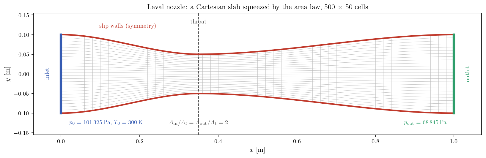
Figure 1: The nozzle and its mesh. The Cartesian slab of 500 x 50 cells is generated in cs_user_mesh_cartesian_define, then every vertex is pulled towards the axis in proportion to the local half height. Faces normal to x stay planar, only the horizontal faces tilt.

Boundary	Location	Nature	Prescribed value
INLET	\(x = 0\)	Compressible subsonic inlet (\(P_t\), \(H_t\))	\(101\,325\) Pa, \(301\,455\) J/kg
OUTLET	\(x = 1\)	Compressible subsonic outlet	\(p = 68\,845\) Pa
WALL	nozzle contour	Slip wall (symmetry)	(none)
SIDES	spanwise planes	Symmetry	(none)

This pair of conditions is the whole point of the case. Nothing prescribes the velocity, the mass flow or the regime: the inlet says what the reservoir holds, the outlet says what pressure the flow must reach, and the solution in between is the answer. Since the flow is inviscid, the nozzle contour is a slip wall imposed as a symmetry, the standard trick for Euler computations.

Numerical setup

Setting	Value	Rationale
Compressible algorithm	pressure-based, constant gamma	code_saturne compressible module
Mesh	\(500 \times 50\) cells (\(\Delta x = 2\) mm)	uniform along the nozzle
Time-stepping	adaptive, max CFL \(= 1\)	pseudo-transient march to the steady state
Iterations	\(8000\)	the field extrema are frozen to five digits well before the end
Convection scheme	1st-order upwind	forced by the compressible module for every variable, whatever the GUI blending factor (cs_cf_model.cpp)
Initialization	\(u = 105\) m/s, \(p = 90\,000\) Pa, \(T = 295\) K	a plausible uniform guess, not the solution

Running the simulation

cd Comp_Laval_Nozzle/

Option A: Graphical interface

code_saturne gui CASE/DATA/setup.xml &

The GUI opens the pre-configured setup.xml. Review the setup if you wish, then launch the run with the gear (Run) button in the toolbar.

Option B: Command line

cd CASE
code_saturne run --n 4

The run takes a few minutes on four cores and writes a time-stamped directory CASE/RESU/<YYYYMMDD-HHMM>/.

Results and verification

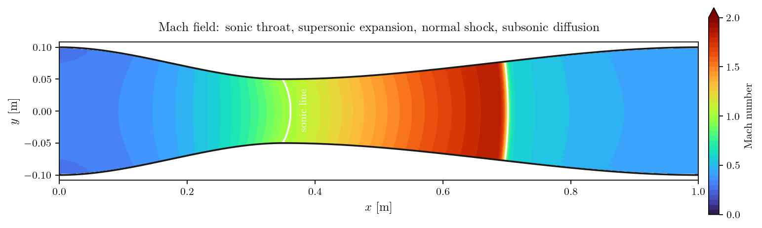
Figure 2: Mach field. The white line is the sonic contour. The flow accelerates through the throat, expands in the divergent, crosses a normal shock and recompresses to the imposed exit pressure.

The section-averaged profiles are compared with the exact quasi-1D solution below. The averaging is mass-flux weighted, which is the meaningful average when the comparison is with a one-dimensional theory.

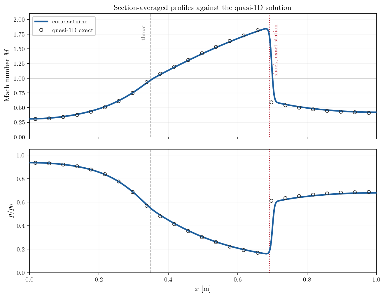
Figure 3: Section-averaged Mach number and static pressure. The symbols are the exact quasi-1D solution for the imposed back pressure. The computed curve lies on it everywhere except across the shock, which any shock-capturing scheme spreads over a few cells.

The agreement is good. The computed profiles lie on the exact solution over the whole isentropic branch, the shock appears where the back pressure says it should, and the flow leaves at the imposed pressure. The choked mass flow, which depends on nothing but the throat being properly sonic, comes out within half a percent of the theoretical value; it can be read directly from the boundary mass flow block of run_solver.log, where the inlet and outlet values also balance, the sign that the pseudo-transient run has reached its steady state.

Two small differences are visible on Figure 3 and are worth naming. The shock stands a few cells downstream of its theoretical station and its peak Mach number is slightly clipped: the compressible module convects at first order, so the front is spread over several cells and settles where the discrete momentum balance closes. And the section-averaged Mach number at the geometric throat falls just short of 1, because in a two-dimensional nozzle the sonic line is curved, as Figure 2 shows, so no plane section is uniformly sonic. That one is a property of the flow rather than of the mesh.

Summary

A single operating point of a Laval nozzle, computed with the compressible module and verified against quasi-1D theory. The regime is set by two boundary conditions and nothing else: total conditions at the inlet, static pressure at a subsonic outlet. The solver chokes the throat at the right mass flow, follows the isentropic branch, and puts the normal shock where the back pressure requires, a few cells from its theoretical station.

The geometry is generated by deforming a Cartesian slab in a user routine, so the case ships without a mesh file and the area law that is verified is the same function that builds the mesh.

References

1. J.D. Anderson. Modern Compressible Flow: With Historical Perspective, 3rd edition, McGraw-Hill, 2003 (chapter 5, quasi-one-dimensional flow).
2. NASA, NACA Report 1135, Equations, Tables and Charts for Compressible Flow, 1953.
3. code_saturne documentation

Authors

Simvia - Questions, remarks and requests are welcome.