Taylor-Couette Flow in a Rotating Frame

Browse this case on GitHub

There are two ways to compute a rotating machine. Either the frame stands still and the walls move through it, or the frame turns with the machine and the equations carry the extra terms that rotation brings. The first is what the mixer tutorials of this section do, with a rotating zone joined to a fixed one. The second is what you reach for when a single blade passage is enough: no interface, no sliding mesh, just a domain that turns and a Coriolis term in the momentum equation.

code_saturne offers that second option from the GUI, as a global angular velocity, and this tutorial exercises it on the one rotating flow that has an exact solution in closed form: the laminar flow between two concentric cylinders.

The same flow is computed twice, once in each frame. That gives two independent verifications for the price of one small mesh: each result is compared with the exact profile, and the two are compared with each other. A rotating frame is a change of variables, nothing more, so once the frame motion is added back the two computations must return the same physical field. If they do not, the extra terms are wrong.

Maintained by Simvia, part of the tutoriel-code_saturne collection.

Learning objectives

After completing this tutorial you will be able to:

1. Put a whole domain in a rotating frame from the GUI, and check in setup.log that the solver has activated the Coriolis source term.
2. Impose a rotating wall, which the GUI cannot express, with a short analytic-function boundary condition.
3. Verify a rotating computation twice: against an exact solution, and by frame invariance.
4. Know where the centrifugal force went, and why the pressure a rotating computation reports is not the physical pressure.

Prerequisites

Requirement	Detail
code_saturne	v9.1
Tutorials	Tbm_Mixer_Vessel_2D (the other way to handle rotation, a rotating zone in a fixed frame)
Background	Rotating frames: Coriolis and centrifugal acceleration

If code_saturne is not yet installed, build it from the official homepage, pull a ready-to-use Singularity image from the Open Simulation Center, or pull the Simvia Docker image before continuing.

Case files

Tbm_Taylor_Couette/
├── CASE_ABSOLUTE/                   # fixed frame, the inner cylinder turns
│   ├── DATA/setup.xml
│   └── SRC/cs_user_boundary_conditions.cpp
├── CASE_ROTATING/                   # frame turning with the inner cylinder
│   ├── DATA/setup.xml
│   └── SRC/cs_user_boundary_conditions.cpp
├── MESH/
│   ├── annulus.msh                  # structured annulus (gmsh)
│   └── annulus.geo                  # its source
├── FIGURES/
└── README.md

The two cases differ by three things only: the frame angular velocity, which cylinder is given a wall velocity, and nothing else. Everything about the fluid, the mesh and the time stepping is identical, which is what makes the comparison between them meaningful.

Physical model

The flow is incompressible, laminar and isothermal, in the annulus between two concentric cylinders. The inner one turns at \(\Omega\), the outer one is at rest. The steady solution is purely azimuthal and depends on the radius alone:

\[ u_\theta(r) = A\,r + \frac{B}{r}, \qquad A = -\frac{\Omega R_1^2}{R_2^2 - R_1^2}, \qquad B = \frac{\Omega R_1^2 R_2^2}{R_2^2 - R_1^2} \]

which satisfies the Navier-Stokes equations exactly, not approximately. The viscous torque on the inner cylinder follows from it in closed form, per unit length:

\[ \mathcal{T} = 4\pi\mu B \]

so the case offers both a profile and a scalar to check.

Flow parameters

Quantity	Symbol	Value	Source in setup.xml
Inner radius	\(R_1\)	\(50\) mm	(geometry)
Outer radius	\(R_2\)	\(100\) mm	(geometry)
Angular velocity	\(\Omega\)	\(1\) rad/s	cs_user_boundary_conditions.cpp, and omega_z for the rotating frame
Density	\(\rho\)	\(1000\) kg/m³	density
Dynamic viscosity	\(\mu\)	\(1\) Pa s	molecular_viscosity
Reynolds number	\(\Omega R_1 d/\nu\)	\(2.5\)	(derived)

The Reynolds number is deliberately small. Above a threshold the circular Couette flow gives way to Taylor vortices, axially periodic rolls that this purely azimuthal solution knows nothing about. At \(Re = 2.5\) the flow is far below that threshold, and the mesh has a single cell across the span in any case, so the rolls could not appear even if they wanted to.

Geometry and boundary conditions

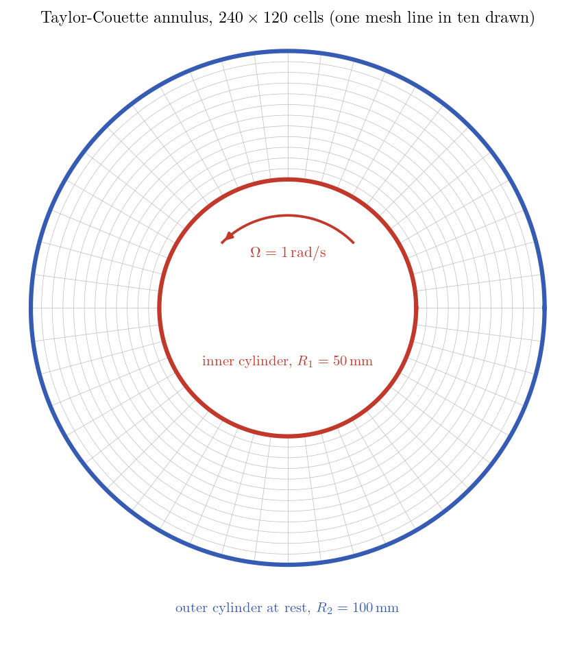
Figure 1: The annulus and its structured mesh. A full annulus has exactly two lateral boundaries, so the case needs neither periodicity nor mesh joining.

The two runs differ only in the frame and in which wall is given a velocity:

Boundary	CASE_ABSOLUTE	CASE_ROTATING
Frame	fixed	rotating at \(\Omega\) about \(z\)
Inner cylinder	wall, \(\mathbf{u} = \mathbf{\Omega} \times \mathbf{r}\)	wall at rest
Outer cylinder	wall at rest	wall, \(\mathbf{u} = -\mathbf{\Omega} \times \mathbf{r}\)
\(z\) planes	symmetry	symmetry

The rotating frame is declared in the GUI as a global angular velocity, under Physical properties. Setting it is enough: the solver reports icorio: 1 (apply Coriolis source terms) in setup.log, together with the rotation axis and rate, and that line is worth checking before trusting a rotating computation.

Why a rotating wall needs a user routine

The GUI can give a wall a velocity, but only a uniform one, three constants. A cylinder turning about its axis needs a velocity that varies from face to face, so it goes through a short analytic function instead:

static void
_rotating_wall(cs_real_t time, cs_lnum_t n_elts, const cs_lnum_t *elt_ids,
               const cs_real_t *coords, bool dense_output, void *input,
               cs_real_t *val)
{
  const cs_real_t omega = *(const cs_real_t *)input;
  const cs_real_3_t *xyz = (const cs_real_3_t *)coords;
  cs_real_3_t *v = (cs_real_3_t *)val;

  for (cs_lnum_t i = 0; i < n_elts; i++) {
    const cs_lnum_t e_id = (elt_ids == nullptr) ? i : elt_ids[i];
    const cs_lnum_t j = dense_output ? i : e_id;

    v[j][0] = -omega*xyz[e_id][1];
    v[j][1] =  omega*xyz[e_id][0];
    v[j][2] =  0.;
  }
}

attached to the zone in cs_user_boundary_conditions_setup:

cs_equation_add_bc_by_analytic(cs_equation_param_by_name("velocity"),
                               CS_BC_DIRICHLET, "inner",
                               _rotating_wall, (void *)&_omega);

The rotating-frame case uses the same function with the opposite sign on the outer cylinder, since a wall at rest in the absolute frame turns backwards in a frame that follows the inner one.

Numerical setup

Setting	Value
Mesh	\(240 \times 120\) cells, one across the span
Turbulence	none, laminar
Time step	\(0.01\) s, constant
Iterations	\(2000\), that is \(20\) s
Viscous time across the gap	\(d^2/\nu = 2.5\) s

Twenty seconds is eight viscous times, so the steady state is reached with a wide margin; the velocity extrema in the log stop moving well before the end.

Running the simulation

cd Tbm_Taylor_Couette/

cd CASE_ABSOLUTE && code_saturne run --n 4 && cd ..
cd CASE_ROTATING && code_saturne run --n 4 && cd ..

Each run takes a few minutes on four cores. The GUI opens either case with code_saturne gui CASE_ABSOLUTE/DATA/setup.xml &.

Results and verification

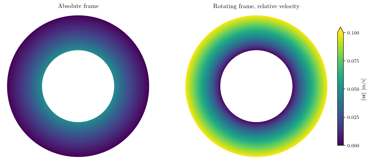
Figure 2: Velocity magnitude, same colour scale. In the absolute frame the fluid is fastest against the inner cylinder that drives it; in the frame turning with that cylinder the picture inverts, the fluid is at rest on the inner wall and sweeps past the outer one. Two different fields, one flow.

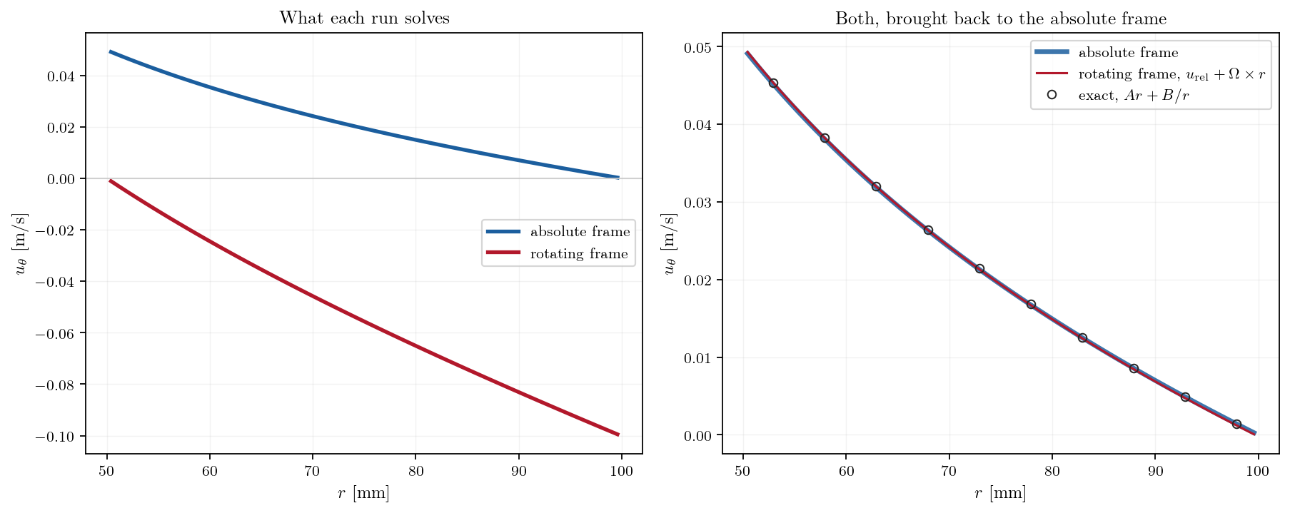
Figure 3: Left, the field each run actually solves: the two have nothing in common, one going to zero at the outer wall and the other at the inner wall. Right, the same two results once the frame motion is added back, against the exact solution.

The agreement is good, and the frame invariance holds: the rotating-frame result, plus \(\mathbf{\Omega} \times \mathbf{r}\), falls back onto the absolute-frame result and onto the exact profile. The torque on the inner cylinder agrees with \(4\pi\mu B\) to a few tenths of a percent in both runs, with the sign it should have, the fluid resisting the rotation.

What remains is discretisation, not a modelling error: halving the cell size halves the residual gap, which is also why the shipped mesh is the finer of the two that were tried.

Where the centrifugal force went

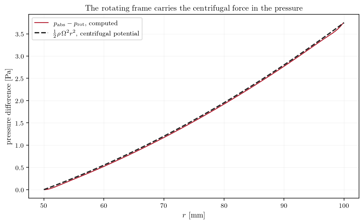
Figure 4: Difference between the pressures computed in the two frames, compared with the centrifugal potential.

A rotating frame introduces two accelerations, Coriolis and centrifugal, but the solver only ever adds the first one: the log says so, apply Coriolis source terms, and the source contains no centrifugal term. The reason is that the centrifugal acceleration is a gradient, so it can be folded into the pressure, and that is what the rotating formulation does.

Figure 4 confirms it: the pressure difference between the two runs follows \(\frac{1}{2}\rho\Omega^2r^2\) over the whole gap. The consequence is practical. In a rotating frame, the pressure the solver writes is a reduced pressure. To recover the physical one, add the centrifugal potential back. Forget it, and a pressure map or an integrated force on a blade will be wrong by a term that grows as the square of the radius.

Summary

The same laminar annular flow, computed in a fixed frame with a rotating wall and in a frame rotating with the inner cylinder. Both match the exact circular Couette profile and the exact viscous torque, and they match each other once the frame motion is added back, which is the check that the rotation terms are right.

Two practical points came out of it. A rotating wall cannot be expressed in the GUI and needs a few lines of analytic boundary condition. And the rotating formulation carries the centrifugal force inside the pressure, so the pressure it reports is not the physical one.

References

1. G.I. Taylor, "Stability of a viscous liquid contained between two rotating cylinders", Philosophical Transactions of the Royal Society A, 223, pp. 289-343, 1923.
2. G.K. Batchelor. An Introduction to Fluid Dynamics, Cambridge University Press, 1967 (section 4.5, steady flow between rotating cylinders).
3. code_saturne documentation

Authors

Simvia - Questions, remarks and requests are welcome.