Balances by Zone (Energy Budget of a Heated Channel)

Browse this case on GitHub

When you run a thermal calculation, the first engineering question is "where does the energy go?": how much enters with the flow, how much the walls supply, how much leaves, and does it all add up. Extracting this by hand from exported fields is tedious and approximate. code_saturne can print this audit itself, exactly, during the run: one call to cs_balance_by_zone gives the term-by-term budget of a variable over any group of cells, and cs_pressure_drop_by_zone does the same for the pressure drop.

This tutorial shows how, on a deliberately simple case where every number can be checked by hand: a laminar channel heated by its walls. The printed budget closes to machine precision, the wall heat input equals the enthalpy gained by the flow, and the temperatures deduced from the tables match the analytic solution.

Maintained by Simvia, part of the tutoriel-code_saturne collection.

Learning objectives

After completing this tutorial you will be able to:

1. Request the budget of a scalar over any zone with cs_balance_by_zone in cs_user_extra_operations.
2. Read the printed table: convective boundary terms, wall (diffusive) terms, internal-boundary terms of a partial zone, unsteady term and closure.
3. Convert the table entries into physical quantities (wall power, enthalpy rise, bulk temperatures).
4. Request a pressure-drop budget with cs_pressure_drop_by_zone and build the mechanical-energy drop from it.
5. Know that zone balances require a uniform time step (a local pseudo-steady time step makes the terms inconsistent).

Prerequisites

Requirement	Detail
code_saturne	v9.1
Background	Basic notions of convective heat transfer

If code_saturne is not yet installed, build it from the official homepage, pull a ready-to-use Singularity image from the Open Simulation Center, or pull the Simvia Docker image before continuing.

Case files

Th_Balance_By_Zone/
├── CASE/
│   ├── DATA/
│   │   └── setup.xml                      # pre-configured GUI case
│   └── SRC/
│       └── cs_user_extra_operations.cpp   # the showcased feature
├── FIGURES/                               # figures used in this README
└── README.md

There is no mesh file: the channel grid is built by code_saturne's internal Cartesian mesher, directly from setup.xml.

Physical model

Air (\(\rho=1.2\ \mathrm{kg\,m^{-3}}\), \(\mu=1.8\times10^{-5}\ \mathrm{Pa\,s}\), \(c_p=1005\ \mathrm{J\,kg^{-1}\,K^{-1}}\), \(k_f=0.025\ \mathrm{W\,m^{-1}\,K^{-1}}\)) enters a plane channel (\(L=1\ \mathrm{m}\), \(H=0.02\ \mathrm{m}\), one cell in \(z\)) at \(U=0.1\ \mathrm{m\,s^{-1}}\) and \(T_0=300\ \mathrm{K}\); both walls are held at \(T_w=340\ \mathrm{K}\). The flow is laminar (\(Re_{D_h}=267\)) and marched with a uniform time step to steady state.

For constant wall temperature the bulk temperature follows the analytic NTU law

\[ T_b(x)=T_w-(T_w-T_0)\,e^{-NTU\,x/L}, \qquad NTU=\frac{h\,P\,L}{\dot m\,c_p}, \]

with \(h\) from the laminar fully developed correlation \(Nu_{D_h}=7.54\), giving \(NTU=3.91\) and an outlet bulk temperature of 339.2 K.

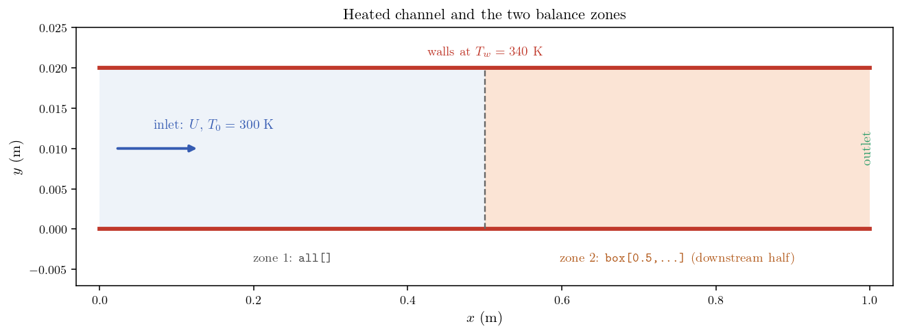
Figure 1: The heated channel and the two zones on which budgets are requested: the whole domain (all[]) and the downstream half (a box[...] selection).

The balances (the feature)

The whole feature is three calls in CASE/SRC/cs_user_extra_operations.cpp, executed at the last time step:

cs_balance_by_zone("all[]", "temperature");
cs_balance_by_zone("box[0.5, -0.1, -0.1, 1.1, 0.1, 0.1]", "temperature");
cs_pressure_drop_by_zone("all[]");

Each call prints a table in run_solver.log. For the scalar budget the entries are the contributions of every mechanism to the zone balance, expressed as \(\rho c_p T\) fluxes integrated over one time step (J per step): boundary convection (Inlet/Outlet), wall diffusion (Smooth W.), internal-boundary convection for partial zones (IB inlet/outlet), the unsteady term, and their Total with a normalized closure indicator.

Two practical points matter:

• Uniform time step required. The entries are per-time-step integrals: with a local (pseudo-steady) time step each face is weighted by its own \(\Delta t\) and the table becomes inconsistent (this case marches to steady state with a true uniform \(\Delta t\) for that reason).
• Dividing by \(\Delta t\) turns entries into powers (W), and dividing a convective entry by \(\dot m\,c_p\,\Delta t\) recovers a bulk temperature.

Numerical setup

Setting	Value
Time scheme	Uniform \(\Delta t=0.005\ \mathrm{s}\), 8000 steps (40 s, steady)
Velocity-pressure algorithm	SIMPLEC
Turbulence	Off (laminar)

Running the simulation

From the tutorial directory:

cd CASE
code_saturne run              # serial
code_saturne run --n 4        # parallel (4 MPI ranks)

The user routine in CASE/SRC/ is compiled automatically; the three balance tables appear at the end of RESU/<id>/run_solver.log.

Results and verification

The budget closes and the wall flux equals the enthalpy rise

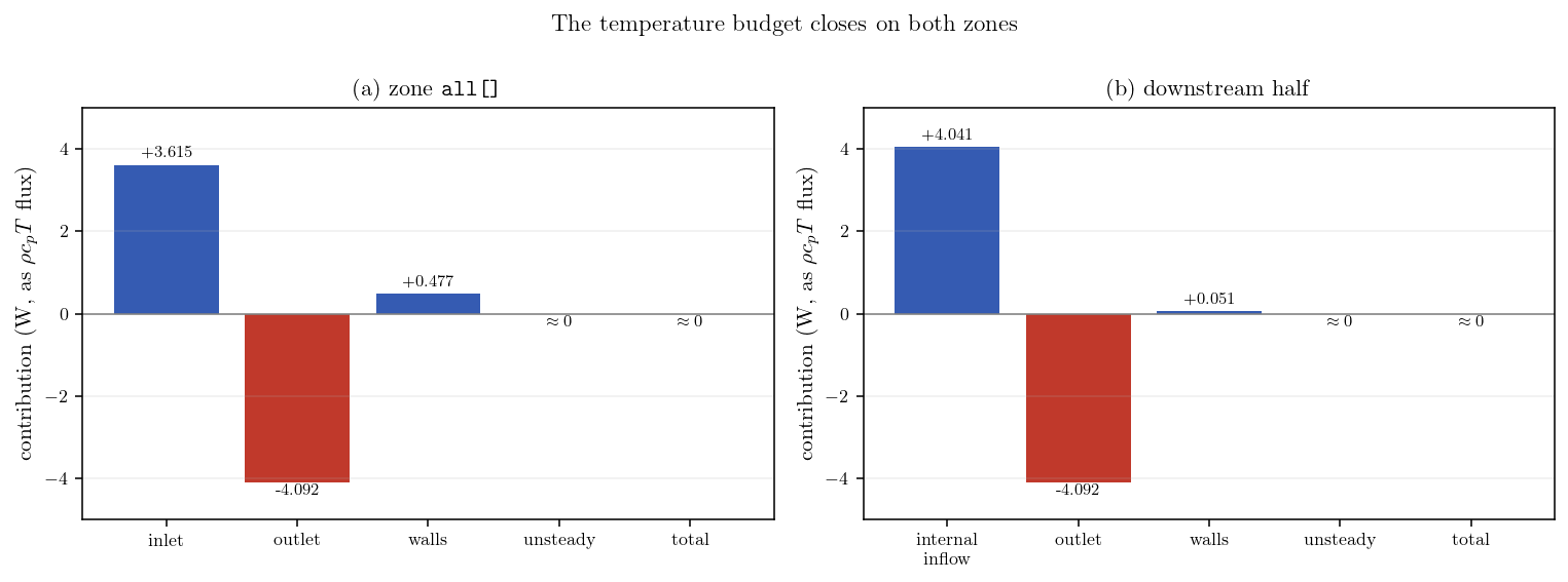
Figure 2: The temperature budget printed by cs_balance_by_zone, converted to watts. On both zones the terms sum to zero (normalized closure $10^{-11}$), and the wall contribution balances the convective deficit exactly.

Quantity (from the tables)	Whole domain	Downstream half
Normalized closure	\(-8\times10^{-12}\)	\(-2\times10^{-12}\)
Wall power	0.4771 W	0.0509 W
Convective enthalpy rise	0.4772 W	0.0510 W

The tables give the physically meaningful numbers

The mean fluid temperature \(T_b(x)\) (the flow-rate-weighted average over a cross-section, i.e. the temperature a perfectly mixed sample would have) rises from 300 K toward the wall temperature along the channel. Dividing a convective entry of a table by \(\dot m\,c_p\,\Delta t\) gives exactly this temperature at the boundary of the zone: 335.1 K at mid-channel (from the downstream-zone table) and 339.3 K at the outlet (from the all[] table), identical to the values computed independently from the exported fields.

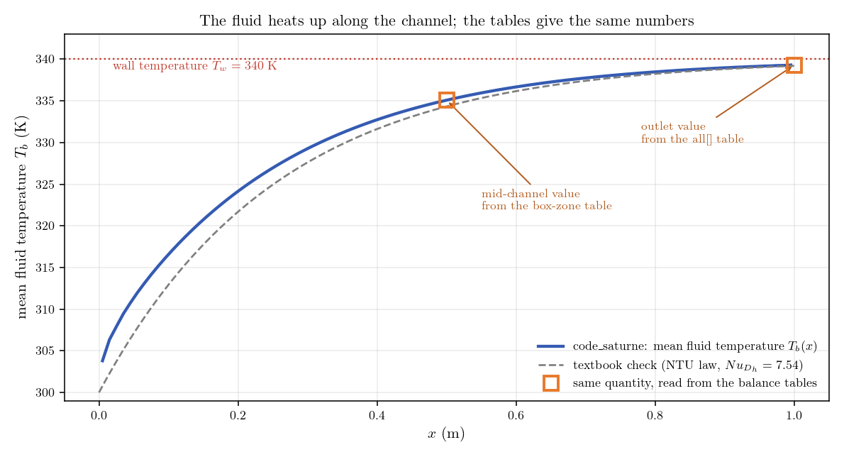
Figure 3: Mean fluid temperature along the channel (blue), heating up toward the 340 K walls. The two orange squares are not computed from the fields: they are read directly from the balance tables, and land exactly on the curve. The dashed line is the textbook NTU check; the small offset in the first half is the thermal entrance region, where the real transfer exceeds the fully developed correlation used by the textbook curve.

Mechanical-energy drop from the pressure-drop table

cs_pressure_drop_by_zone prints the boundary integrals of \(p\,u\), of \(\tfrac12\rho u^2\,u\) and of the flow rate. Combining them gives the drop of mechanical energy per unit flow rate:

\[ \Delta\Big(p+\tfrac{\rho u^2}{2}\Big) =\frac{[\,\int(p+\tfrac12\rho u^2)\,\mathbf{u}\cdot\mathrm{d}\mathbf{S}\,]_{\mathrm{in}}^{\mathrm{out}}}{Q} =0.0547\ \mathrm{Pa}, \]

against \(12\,\mu\,U\,L/H^{2}=0.054\ \mathrm{Pa}\) for developed Poiseuille flow (1.3 percent, the small excess being the entrance loss). Note that the static pressure drop alone would not match, because part of the inlet pressure is converted into the kinetic energy of the developing parabolic profile.

Summary

This tutorial audited the energy of a thermal calculation with three calls in cs_user_extra_operations: the temperature budget over the whole channel and over its downstream half, and the pressure drop over the domain. The tables close to machine precision, the wall flux equals the convective enthalpy rise on both zones, the bulk temperatures recovered from the tables match the offline averages exactly and follow the analytic NTU law, and the mechanical-energy drop matches Poiseuille within 1.3 percent. Zone balances are the quickest rigorous check of a thermal calculation (where does the energy enter, leave, accumulate), with one caveat: they require a uniform time step.

References

1. code_saturne documentation: https://code-saturne.org/doc/.
2. F. P. Incropera, D. P. DeWitt, T. L. Bergman, and A. S. Lavine, Fundamentals of Heat and Mass Transfer, Wiley.

Authors

Simvia - Questions, remarks and requests are welcome.