Dam Break with a Bottom Obstacle (VOF)

Browse this case on GitHub

This tutorial simulates the gravity-driven collapse of a water column inside a two-dimensional tank. The liquid front propagates across the dry section of the tank, impacts a rectangular obstacle, rises along its upstream face, and subsequently overtops it. The case is designed as a compact demonstration of free-surface flow modelling with the homogeneous Volume-of-Fluid (VOF) model in code_saturne.

The supplied setup is configured for code_saturne 9.1 and uses a water-air mixture without interphase mass transfer.

Maintained by Simvia, part of the tutoriel-code_saturne collection.

Learning objectives

After completing this tutorial, the user should be able to:

1. Activate the homogeneous VOF model for an incompressible water-air flow.
2. Initialize two phases in different volume zones using the void_fraction field.
3. Define phase-dependent density and dynamic viscosity.
4. Include gravity and surface-tension effects.
5. Run a transient free-surface calculation with a fixed time step.
6. Visualize the interface from the VOF field and assess the main stages of the dam-break motion.

Prerequisites

Requirement	Detail
code_saturne	v9.1
Background	Basic notions of multiphase modelling with the VOF method

If code_saturne is not yet installed, build it from the official homepage, pull a ready-to-use Singularity image from the Open Simulation Center, or pull the Simvia Docker image before continuing.

Case files

Vof_Dam_Break/
├── CASE/
│   └── DATA/
│       └── setup.xml
├── MESH/
│   └── damBreak_with_groups.med
├── FIGURES/                   # figures used in this README
└── README.md

Physical model

Homogeneous two-phase formulation

The case uses the homogeneous VOF model with no interphase mass transfer. Both phases share a single velocity field and a single pressure field. The interface is represented by the scalar field

\[ \alpha = \texttt{void\_fraction}, \]

where, in this case:

• \(\alpha=0\) represents water.
• \(\alpha=1\) represents air.
• \(0<\alpha<1\) identifies cells crossed by the numerically captured interface.

The phase indicator is transported in conservative form. In the VOF formulation, the transport equation may be written as

\[ \frac{\partial \alpha}{\partial t} + \nabla\cdot(\alpha\mathbf{u}) + \nabla\cdot\left[\alpha(1-\alpha)\mathbf{u}_r\right] =0, \]

where \(\mathbf{u}\) is the mixture velocity and \(\mathbf{u}_r\) represents the interface-compression or drift contribution used by the VOF discretization. The right-hand side is zero because vaporization, condensation, and other phase-change mechanisms are disabled.

The local mixture properties are obtained from the volume fraction:

\[ \rho=(1-\alpha)\rho_w+\alpha\rho_a, \]

\[ \mu=(1-\alpha)\mu_w+\alpha\mu_a, \]

where subscripts \(w\) and \(a\) denote water and air, respectively.

Momentum equation

The incompressible variable-density momentum equation is solved for the mixture:

\[ \frac{\partial(\rho\mathbf{u})}{\partial t} +\nabla\cdot(\rho\mathbf{u}\otimes\mathbf{u}) =-\nabla p +\nabla\cdot\left[\mu\left(\nabla\mathbf{u}+\nabla\mathbf{u}^{T}\right)\right] +\rho\mathbf{g} +\mathbf{f}_{\sigma}, \]

where \(\mathbf{g}\) is gravity and \(\mathbf{f}_{\sigma}\) is the surface-tension force. Surface tension is represented through the continuum-surface-force approach implemented by code_saturne.

The turbulence model is disabled. The calculation is therefore performed as a laminar, transient two-phase simulation.

Flow parameters

The two phases are initialized at rest. The motion is generated entirely by gravity after the idealized instantaneous removal of the gate retaining the water column.

Parameter	Water	Air	Unit	Source in setup.xml
Density \(\rho\)	1000	1	\(\mathrm{kg\,m^{-3}}\)	density/value_0, value_1
Dynamic viscosity \(\mu\)	\(1.0\times10^{-3}\)	\(1.48\times10^{-5}\)	\(\mathrm{Pa\,s}\)	molecular_viscosity/value_0, value_1

Additional physical parameters are:

Parameter	Value	Unit	Source in setup.xml
Surface tension \(\sigma\)	0.07	\(\mathrm{N\,m^{-1}}\)	surface_tension
Gravity	\((0,-9.81,0)\)	\(\mathrm{m\,s^{-2}}\)	gravity/gravity_y
Initial velocity	\((0,0,0)\)	\(\mathrm{m\,s^{-1}}\)	velocity/initialization
Reference pressure	101325	Pa	reference_pressure
Reference temperature	293.15	K	reference_temperature

Geometry and boundary conditions

Geometry

The domain is a square tank, \(0.584\times0.584\ \mathrm{m}\), one cell thick in the spanwise direction. A rectangular obstacle (\(0.024\ \mathrm{m}\) wide, \(0.048\ \mathrm{m}\) tall) sits on the floor with its leading edge at \(x=0.292\ \mathrm{m}\). The initial water column occupies the bottom-left corner, \(0.1461\ \mathrm{m}\) wide and \(0.292\ \mathrm{m}\) tall; the rest of the tank is air (see Figure 1 for the mesh and boundary layout).

The two phases are set in setup.xml by initializing the whole domain with \(\alpha=1\) (air), then the water-column zone (\(0\le x\le0.1461\), \(0\le y\le0.292\)) with \(\alpha=0\) (water).

Mesh

The MED mesh is a structured five-block mesh extruded through one cell in the spanwise direction. It contains:

• 2268 hexahedral cells.
• 4746 vertices.
• One cell across the quasi-2D thickness.
• Local refinement around the bottom obstacle and the lower part of the tank.

The front and back planes are symmetry boundaries, so the solution is effectively two-dimensional.

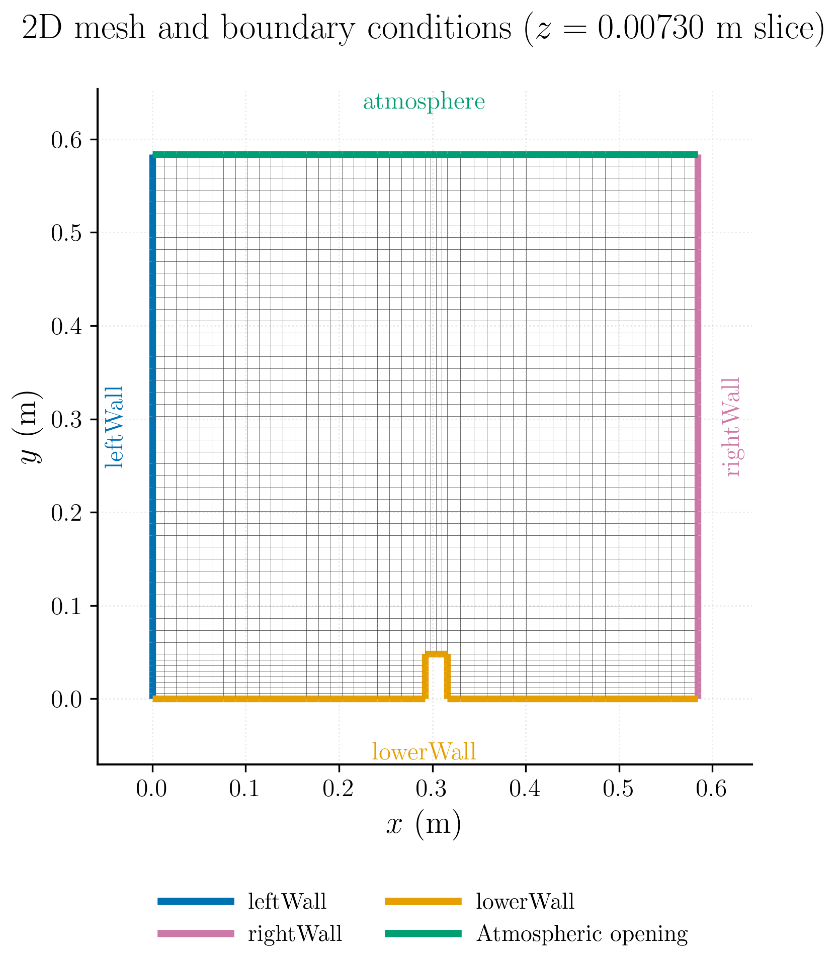
Figure 1: Mesh and boundary conditions (z = 0.00730 m slice).

Boundary conditions

Boundary zone	Type	Definition
leftWall	Wall	No-slip velocity
rightWall	Wall	No-slip velocity
lowerWall	Wall	No-slip velocity; includes the tank floor and obstacle
atmosphere	Outlet	Free outlet at the tank top
front	Symmetry	Quasi-2D plane
back	Symmetry	Quasi-2D plane

The top of the tank (atmosphere) is a standard outlet (imposed reference pressure, zero-gradient velocity) through which air leaves as the water sloshes up. It is not a rigorously open in/outflow boundary, but the net flux through the top stays small, so a plain outlet is adequate here and needs no user routine.

Numerical setup

The main numerical settings stored in CASE/DATA/setup.xml are summarized below.

Setting	Value
code_saturne setup version	9.1
Calculation type	Unsteady
Velocity-pressure coupling	SIMPLEC
Time step	\(2.5\times10^{-4}\ \mathrm{s}\)
Number of time steps	3000
Final simulated time	0.75 s
Turbulence model	Off
VOF model	Homogeneous mixture, no mass transfer

Three probes are also defined at the mid-thickness plane:

Probe	\(x\) (m)	\(y\) (m)	\(z\) (m)
1	0.06983	0.14371	0.00730
2	0.27296	0.02700	0.00730
3	0.30700	0.06714	0.00730

They can be used to monitor the local pressure, velocity, and phase indicator during the collapse and obstacle impact.

The fixed time step should be checked against the maximum Courant number reported by code_saturne. A finer mesh or a more violent interface motion may require a smaller value.

Running the simulation

The commands below start from the tutorial directory:

cd Vof_Dam_Break/

Option A: Graphical interface

code_saturne gui CASE/DATA/setup.xml &

The GUI opens the pre-configured setup.xml. Review the setup if you wish, then launch the run with the gear (Run) button in the toolbar. To run in parallel, set the number of processes under Calculation management > Performance settings before launching.

Option B: Command line

The command-line launcher is run from inside the case directory:

cd CASE

# serial
code_saturne run

# parallel (e.g. 4 MPI ranks)
code_saturne run --n 4

The mesh is light, so the case runs quickly; serial runs easily.

Each run creates a time-stamped directory CASE/RESU/<YYYYMMDD-HHMM>/ containing:

• run_solver.log: solver log and residual history,
• monitoring/: probe time series (probes_*.csv),
• postprocessing/: volume and boundary fields in EnSight Gold format.

Results and verification

Interface evolution

The void_fraction field is post-processed at four instants. Water is dark, air is light, and the intermediate shades show the numerically captured interface. The obstacle (grey) is at \(x/a=2\), using the initial column width \(a=0.1461\ \mathrm{m}\) as length scale.

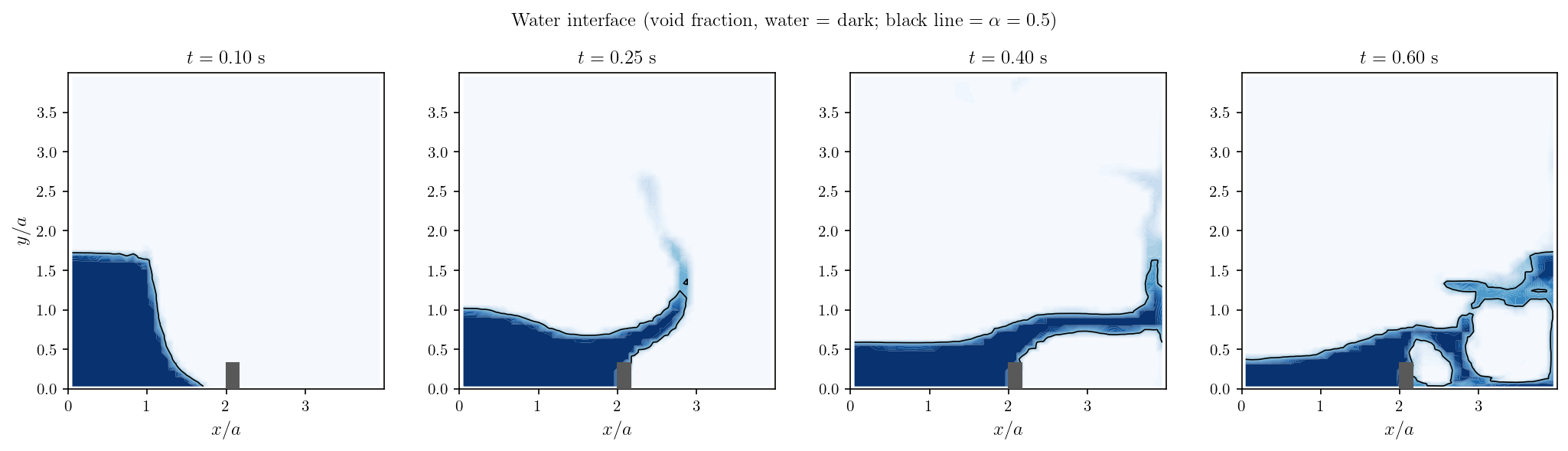
Figure 2: Interface evolution. The column collapses and the surge front advances along the floor (0.10 s), impacts the obstacle and forms a rising jet (0.25 s), overtops it (0.40 s), and surges downstream while entrapping an air pocket under the overturning sheet (0.60 s).

The snapshots reproduce the expected sequence for a dam break interacting with a bottom obstacle: gravity-driven collapse, propagation of the surge front along the floor, impact on the obstacle and jet formation, overtopping, and air entrapment under the overturning sheet. The verification here is qualitative: the purpose of this tutorial is to show a complete, reproducible VOF set-up (model, phases, initialization, boundary conditions), not to provide a quantitative benchmark.

Summary

This tutorial set up a gravity-driven dam break with a bottom obstacle using the homogeneous VOF model of code_saturne: water-air mixture properties, void-fraction initialization of the water column with the flow at rest, surface tension and gravity, and a free outlet at the tank top. The interface evolution reproduces the expected stages (collapse, floor surge, obstacle impact, jet, overtopping and air entrapment). It is meant as a reproducible VOF set-up example rather than a validated benchmark: the mesh is intentionally coarse, the flow is treated as quasi-2D, and the verification is qualitative. It is a good starting point for more advanced free-surface simulations.

References

1. code_saturne documentation, VOF model for free-surface or dispersed flow, homogeneous-mixture modelling module: https://www.code-saturne.org/documentation/9.0/doxygen/src/group__vof.html.
2. C. W. Hirt and B. D. Nichols, “Volume of Fluid (VOF) Method for the Dynamics of Free Boundaries,” Journal of Computational Physics, vol. 39, no. 1, pp. 201-225, 1981. https://doi.org/10.1016/0021-9991(81)90145-5.
3. J. U. Brackbill, D. B. Kothe, and C. Zemach, “A Continuum Method for Modeling Surface Tension,” Journal of Computational Physics, vol. 100, no. 2, pp. 335-354, 1992. https://doi.org/10.1016/0021-9991(92)90240-Y.
4. S. Koshizuka and Y. Oka, “Moving-Particle Semi-Implicit Method for Fragmentation of Incompressible Fluid,” Nuclear Science and Engineering, vol. 123, no. 3, pp. 421-434, 1996. https://doi.org/10.13182/NSE96-A24205.
5. code_saturne documentation

Authors

Simvia - Questions, remarks and requests are welcome.