Mesh Convergence with csauto

Browse this case on GitHub

A mesh convergence study is the same case run several times on finer and finer meshes, until the answer stops moving. The work is not in the physics, it is in the bookkeeping: four case directories to create, four runs to launch and follow, four sets of results to line up, and the certainty that nothing else changed along the way.

csauto does that bookkeeping. You give it one template case and one CSV with one row per case, it writes the case directories, launches them, and shows the campaign in a web dashboard. This tutorial runs the cavity of Th_Buoyant_Cavity on \(20^2\), \(40^2\), \(80^2\) and \(160^2\) cells and reads the mesh convergence off the result.

csauto orchestrates the campaign and shows whether each run converged. The physical comparison at the end is ordinary post-processing of the volume output, done once the campaign is over.

Maintained by Simvia, part of the tutoriel-code_saturne collection.

Learning objectives

After completing this tutorial you will be able to:

1. Turn an existing case into a csauto template by replacing the values you want to vary with placeholders.
2. Write a DOE table where the parameters that must follow the mesh do follow it.
3. Launch a campaign with csauto prepare and csauto run, and read its state in the dashboard.
4. Check, before comparing anything, that every run in the campaign actually converged.
5. Extract a convergence order from the campaign, and tell a global measure from a local one.

Prerequisites

Requirement	Detail
code_saturne	v9.1
csauto	v0.5.0
Docker	the runtime used here, so no local code_saturne build is needed
Tutorials	Th_Buoyant_Cavity, the case this campaign varies
Background	Notions of grid convergence and of Richardson extrapolation

csauto is free software under the GPL and lives at github.com/simvia-tech/csauto, with a landing page and its own documentation. It needs Python 3.11 or later and installs in one line, which clones it to ~/.local/share/csauto, creates a virtual environment and adds the csauto alias to your shell:

bash -c "$(curl -fsSL https://raw.githubusercontent.com/simvia-tech/csauto/main/install.sh)"
source ~/.bashrc   # or: source ~/.zshrc

Re-running the same line updates an existing installation. Check what you have with:

csauto --version

csauto is before its 1.0 release and says so: expect its commands to move a little. The version used throughout is 0.5.0.

If code_saturne is not yet installed, this tutorial needs no local build: the Docker image is pulled on the first run. To install it anyway, build it from the official homepage, pull a ready-to-use Singularity image from the Open Simulation Center, or pull the Simvia Docker image.

Case files

Csa_Mesh_Convergence/
├── TEMPLATE/
│   └── DATA/
│       └── setup.xml       # the cavity case, with placeholders
├── csauto.toml             # runtime and dashboard settings
├── doe.csv                 # one row per case
├── FIGURES/
└── README.md

RUNS/, the four case directories csauto generates, is not shipped: it is rebuilt by csauto prepare.

The template

The template is the CASE of Th_Buoyant_Cavity, at \(Ra = 10^5\), with three values replaced by {placeholder} names. csauto substitutes them line by line, so a placeholder works anywhere in setup.xml, including inside an attribute:

<mesh_cartesian>
  <x_direction ncells="{n}" min="0.0" max="1.0" prog="1.0" law="constant"/>
  <y_direction ncells="{n}" min="0.0" max="1.0" prog="1.0" law="constant"/>
  <z_direction ncells="1" min="0.0" max="1.0" prog="1.0" law="constant"/>
</mesh_cartesian>

<iterations>{iterations}</iterations>

<profile label="centerline">
  <var_prop name="velocity" component="0"/>
  <var_prop name="temperature"/>
  <format name="CSV"/>
  <output_type>end</output_type>
  <points>{points}</points>
  <snap_mode>none</snap_mode>
  <interpolation>yes</interpolation>
  <formula>x = 0.5;
y = s;
z = 0.5;</formula>
</profile>

The mesh is built by code_saturne's own Cartesian mesher, so refining it is a matter of one number and there is no mesh file to regenerate. The profile writes the vertical centreline to RESU/<run>/profiles/centerline.csv, which the dashboard can plot.

The DOE table

case_id,n,iterations,points
case_020,20,2000,21
case_040,40,2000,41
case_080,80,2000,81
case_160,160,4000,161

Only one thing is being studied, the mesh, but two other columns have to follow it.

The iteration budget. The case reaches its steady state with a local (pseudo) time step capped by a Courant number of one, so the time step follows the cell size: a finer mesh advances less per iteration and needs more of them. Left at \(2000\) iterations for every mesh, the \(160^2\) run is still moving when it stops, and the study then compares a converged coarse solution with an unconverged fine one. Doubling the budget for the finest mesh settles it.

The profile resolution. The profile is sampled at fixed coordinates, so asking for \(200\) points on a \(20\)-cell mesh gives ten identical samples per cell and a staircase. One point per cell face keeps every mesh sampled at its own resolution.

case_id is free, with one catch: csauto's bulk commands look for directories whose name starts with case, so case_020 is seen by csauto doctor and csauto run while mesh_020 would not be.

Step 1: tell csauto how to run

Everything below is run from the tutorial directory, because that is where csauto looks for its configuration:

cd Csa_Mesh_Convergence

csauto.toml is picked up automatically from the current directory, so these settings apply to every command that follows and none of them has to be repeated on the command line:

runtime = "docker"
docker_image = "simvia/code_saturne:9.1.0"
use_slurm = false
max_parallel = 4
host = "127.0.0.1"
port = 8000

Key	What it does
runtime	how to launch the solver: docker, singularity, native for a local build, or auto to let csauto pick
docker_image	the image used by the docker runtime, here the Simvia image for code_saturne 9.1
use_slurm	false runs the cases as background processes on this machine; true submits one Slurm job per case
max_parallel	how many cases may run at the same time. Four is the size of this campaign, so all four start at once
host, port	where the dashboard listens. 127.0.0.1 keeps it on this machine

Choosing docker is what makes the tutorial reproducible without a local build. If you already have code_saturne installed, replace those two lines with runtime = "native" and saturne_bin = "/path/to/code_saturne".

Step 2: generate the four cases

csauto prepare doe.csv TEMPLATE RUNS
csauto doctor RUNS

prepare writes RUNS/case_020/ to RUNS/case_160/, each with its rendered setup.xml and a doe_row.csv recording the values used. It warns that the shared MESH and POST directories are missing, which is expected here: the mesh is in setup.xml. doctor then checks the runtime and the cases before anything is launched, and prints one [OK] per check:

[OK] write OK: RUNS
[OK] 4 cases detected
[OK] setup.xml present in every case
[OK] docker available

Step 3: open the dashboard

csauto serve RUNS

The host and port come from csauto.toml, so there is nothing to pass here. The command stays in the foreground for the rest of the session: run it in its own terminal, then open http://127.0.0.1:8000. On a remote machine, tunnel the port first with ssh -L 8000:127.0.0.1:8000 your-server.

The dashboard is worth a look before committing four runs to the queue, because it can show what prepare produced. Scroll to Side-by-Side Comparison, pick two cases, and choose setup.xml as the file:

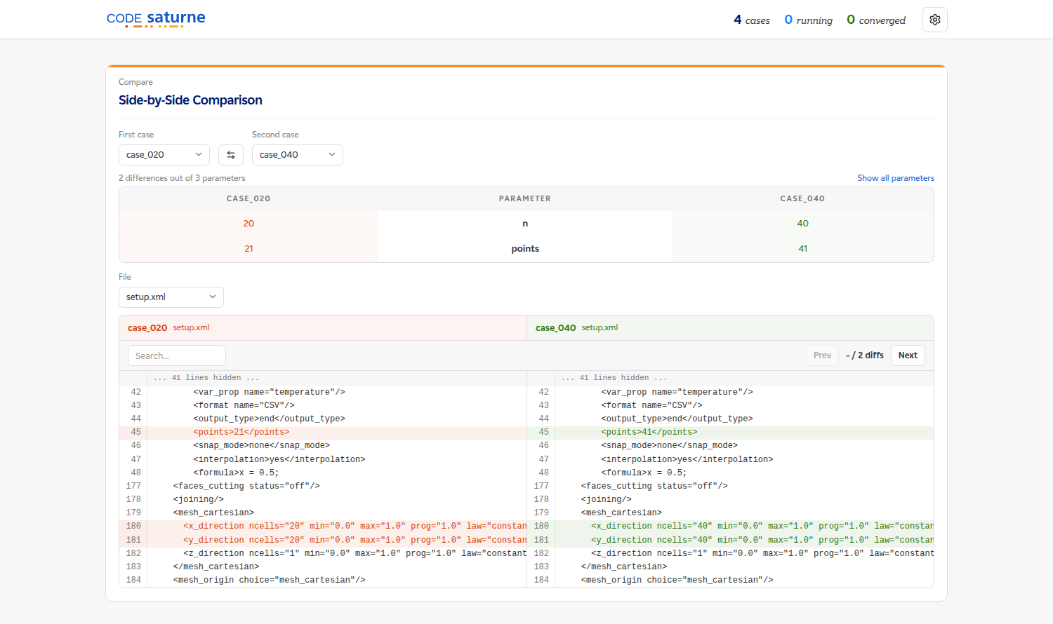
Figure 1: Two prepared cases compared. The parameter table names what differs, and the file diff shows where: the two ncells attributes and the profile resolution. Everything else in the 274 lines of setup.xml is identical.

Step 4: launch the campaign from the dashboard

This is the recommended way to launch: the Status panel does it, and you stay in the interface you will be watching anyway.

1. Click the checkbox in the table header to select all four cases. The toolbar then reads 4 selected and its buttons become active.
2. Click Run. A dialog asks for the three numbers csauto needs.
3. Set MPI Ranks (n) to 4 and leave OMP Threads (nt) at 1, so each case gets four ranks with one thread each. Max Parallel comes pre-filled at 4, which is what we want here: all four at once, for sixteen cores in total.
4. Click Run.

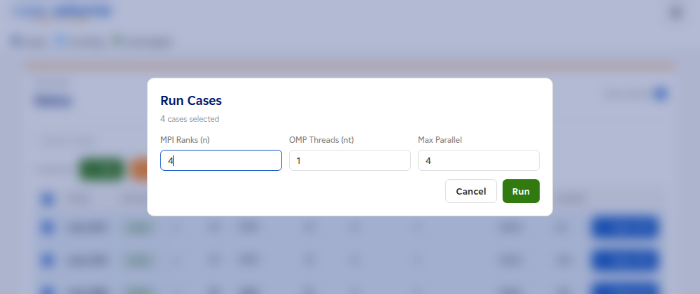
Figure 2: Launching the four cases from the Status panel.

The rows go from PREPARED to RUNNING, the LAST ITER column climbs as each solver advances, and each row turns DONE on its own.

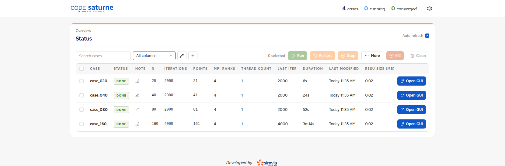
Figure 3: The Status panel once the campaign is over. The DOE columns sit next to the case name, so the mesh, the iteration budget and the profile resolution are visible with the state of each run.

The whole campaign is over in the time of its longest case: \(6\) s, \(24\) s, \(52\) s and \(3\) min \(14\) s of wall time, all four at once.

The same launch from a terminal, for a script or a machine with no browser, is:

csauto run "$PWD/RUNS" --n 4 --nt 1

Note the absolute path: the launcher needs one, which is what "$PWD/RUNS" is for. The command returns as soon as the cases are launched, since they run in the background either way.

Step 5: check that every run converged

This is the step to do before looking at any physics. A mesh convergence study compares four steady solutions, and a run that stopped short of steady state is not one of them.

In the Residuals Plot panel, leave the case selector on All (4): the four runs are overlaid on one chart.

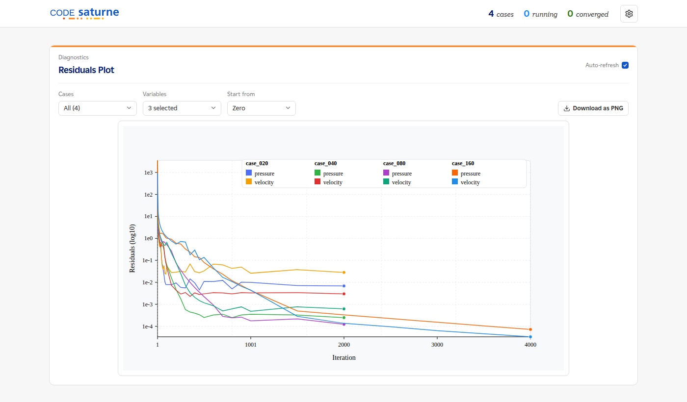
Figure 4: Residuals for the four runs on one chart. The two longest curves are the 160² case, which was given 4000 iterations.

Each run falls by several orders of magnitude and flattens. The coarsest mesh flattens highest, near \(3\times10^{-2}\) on the velocity, and its near-wall probe still wanders by \(0.7\%\) over the last 200 iterations, which the Probes panel shows and RESU/<run>/monitoring/ records: on \(20^2\) cells the flow does not fully settle. The other three settle to better than \(0.01\%\). That is worth knowing before the coarse point is read as an error of discretisation alone.

Step 6: read what the campaign cost

The Timing Snapshot panel reads each run's performance.log and puts the four side by side, with a Download as CSV button for the numbers.

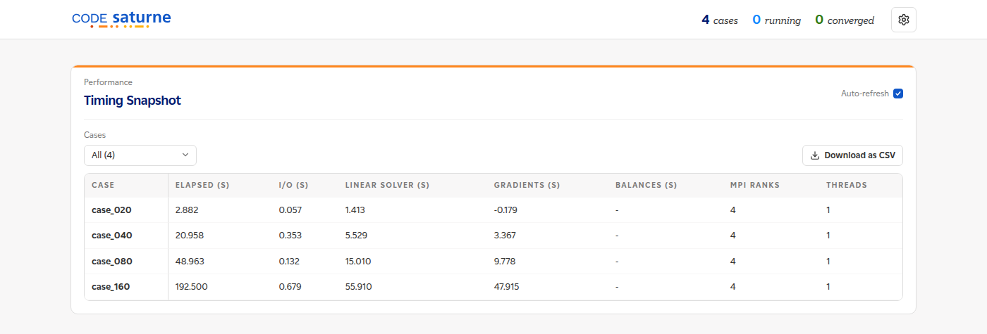
Figure 5: Solver time per case, from each run's own performance log.

Mesh	Cells	Iterations	Elapsed
\(20^2\)	\(400\)	\(2000\)	\(2.9\) s
\(40^2\)	\(1\,600\)	\(2000\)	\(21.0\) s
\(80^2\)	\(6\,400\)	\(2000\)	\(49.0\) s
\(160^2\)	\(25\,600\)	\(4000\)	\(192.5\) s

Four times the cells and twice the iterations cost roughly four times the time between the last two meshes. That ratio is the reason a convergence study stops somewhere, and the reason it is worth knowing where.

Step 7: compare the meshes

The comparison itself is ordinary post-processing, done after the campaign on the volume output of each run: the horizontal velocity is sampled along the vertical centreline of the cavity, at the same \(400\) points for all four meshes.

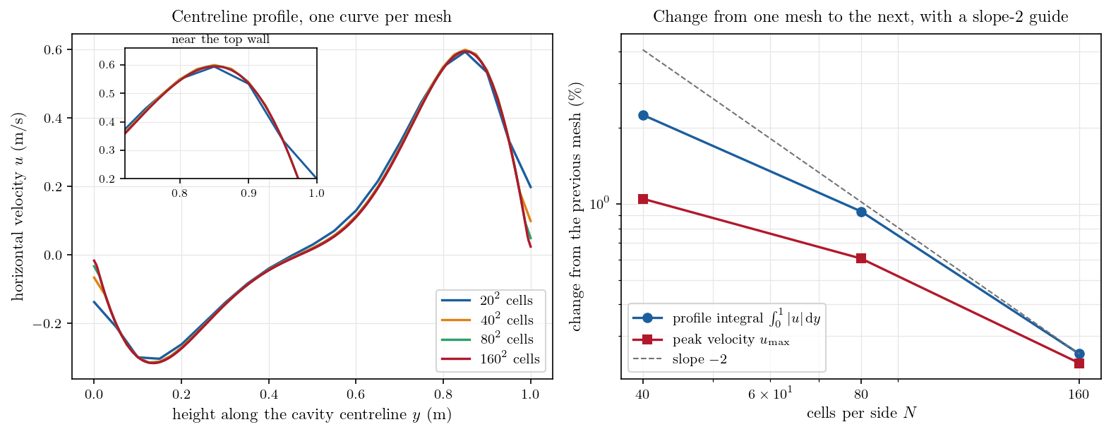
Figure 6: Left, the centreline profile on each mesh, with the near-wall peak magnified. Right, how much each measure moves from one mesh to the next.

Mesh	\(\int_0^1 \lvert u \rvert \, \mathrm{d}y\)	change	\(u_{\max}\)	change
\(20^2\)	\(0.246926\)		\(0.593774\)
\(40^2\)	\(0.241371\)	\(2.25\%\)	\(0.599993\)	\(1.05\%\)
\(80^2\)	\(0.239118\)	\(0.93\%\)	\(0.596348\)	\(0.61\%\)
\(160^2\)	\(0.238508\)	\(0.25\%\)	\(0.594952\)	\(0.23\%\)

The profiles are already close on \(40^2\) cells and indistinguishable by eye from \(80^2\) on. What separates the meshes is the peak near the top wall, where the boundary layer is thin, which is where the magnified inset looks.

The integral of the profile is a global measure and it converges cleanly: the change shrinks by a factor of \(2.4\) and then \(3.7\) as the cell size is halved, approaching the factor of four a second-order scheme gives, and the observed order over the three finest meshes is \(1.89\). The peak velocity is a local measure taken inside a boundary layer, and it shrinks at about the same rate but not monotonically, overshooting on \(40^2\) before settling. Reading an order of convergence off a local extremum is unreliable for that reason.

For engineering purposes the answer is that \(80^2\) cells are enough: going to \(160^2\) moves both measures by a quarter of a percent. This is a self-convergence study: it says when the mesh stops mattering, not whether the physics is right. The comparison against the reference solution of Sockol lives in Th_Buoyant_Cavity.

Summary

One template, one CSV of four rows, two commands. csauto wrote the four cases, ran them side by side, and showed in one dashboard that each had converged, what each had cost, and that nothing but the intended parameters differed between them.

The two things worth carrying over to the next campaign are in the DOE table. A parameter that must follow the mesh belongs in its own column, or the campaign compares solutions that are not comparable: here the iteration budget, because the local time step follows the cell size, and the profile resolution, because a profile sampled far finer than the mesh only shows the mesh. And the convergence of each run is worth checking before any of the results are compared.

References

1. csauto, the campaign tool used here, and its documentation
2. P. J. Roache, Verification and Validation in Computational Science and Engineering, Hermosa, 1998, for grid convergence and Richardson extrapolation
3. code_saturne documentation

Authors

Simvia - Questions, remarks and requests are welcome.