ALE Piston in a Duct (Moving Mesh)

Browse this case on GitHub

Most CFD boundaries stand still. Some do not: a valve closes, a piston sweeps a cylinder, a hull heaves, a blade flutters. When the boundary moves, the mesh has to move with it, and the conservation equations have to be written for cells that change shape and volume as they are integrated. That is what the Arbitrary Lagrangian-Eulerian formulation provides: the mesh follows the boundary, the solver accounts for the volume it sweeps, and the fluid never notices a discontinuity.

Two things then need care, and neither is physics. The mesh has to deform gracefully, which means deciding how the prescribed motion of one boundary is distributed over the interior, and the other boundaries have to be told whether they may move, slide, or stay put. Get the second one wrong and the mesh simply refuses to budge.

This tutorial pushes a piston into a duct along a prescribed law and checks the result against the exact solution, which this configuration happens to have in closed form. The whole case is set up from the GUI: there is no user routine at all.

Maintained by Simvia, part of the tutoriel-code_saturne collection.

Learning objectives

After completing this tutorial you will be able to:

1. Activate the ALE method and prescribe the motion of a boundary from the GUI, with no user routine.
2. Set the ALE condition on the remaining boundaries so that the mesh can actually deform, and recognise the prescribed-velocity option that the solver accepts but does not apply.
3. Verify a moving-mesh computation against an exact solution: the boundary law, the fluid velocity, the unsteady pressure drop, and the way the deformation is spread over the interior.

Prerequisites

Requirement	Detail
code_saturne	v9.1
Tutorials	any of the 00_foundations laminar cases
Background	Incompressible flow, transient simulation

If code_saturne is not yet installed, build it from the official homepage, pull a ready-to-use Singularity image from the Open Simulation Center, or pull the Simvia Docker image before continuing.

Case files

Ale_Piston_Duct/
├── CASE/
│   └── DATA/
│       └── setup.xml     # the whole case, GUI-authored
├── FIGURES/              # figures used in this README
└── README.md

CASE/SRC/ is empty on purpose: everything here, including the piston law, is expressed in the GUI. The duct is built by the internal Cartesian mesher, so there is no mesh file either.

Physical model

The flow is incompressible, laminar and isothermal. The duct is closed at one end by the piston and open at the other, and its side walls are slip, which is the choice that makes the case exactly solvable: with no shear at the walls the flow stays one-dimensional, and the viscosity drops out of the solution altogether.

Parameter	Value	Source
Density \(\rho\)	1 kg/m³	setup.xml: density
Dynamic viscosity \(\mu\)	\(10^{-3}\) Pa·s	setup.xml: molecular_viscosity
Duct length \(L_0\)	1 m	mesh
Duct height	0.2 m	mesh
Piston stroke speed \(V_0\)	0.2 m/s	setup.xml: piston ale formula
Ramp time \(\tau\)	0.2 s	idem

The piston is started smoothly rather than jerked into motion, following

\[d(t) = V_0\left[t - \tau\left(1 - e^{-t/\tau}\right)\right], \qquad V(t) = V_0\left(1 - e^{-t/\tau}\right)\]

so that its velocity rises from zero and settles at \(V_0\). The ramp is what makes the pressure check below interesting: it gives a decaying acceleration to measure.

The exact solution

The fluid is incompressible and the duct has one open end, so all the fluid displaced by the piston leaves through the outlet and the velocity is uniform:

\[u(x,t) = V(t)\]

The momentum equation then reduces to \(\partial p/\partial x = -\rho\, \mathrm{d}V/\mathrm{d}t\), and the pressure drop over the remaining length \(L(t) = L_0 - d(t)\) is pure unsteady inertia:

\[\Delta p(t) = \rho\, L(t)\, \frac{\mathrm{d}V}{\mathrm{d}t}\]

Three exact quantities, then, and none of them involves the mesh: they are what the ALE machinery has to reproduce.

Geometry and boundary conditions

Boundary	Flow condition	ALE condition
piston (\(x=0\))	Wall	prescribed displacement
outlet (\(x=L_0\))	Outlet	fixed
lateral (\(y=\pm 0.1\))	Symmetry (slip)	sliding
frontback (\(z\) planes)	Symmetry	sliding

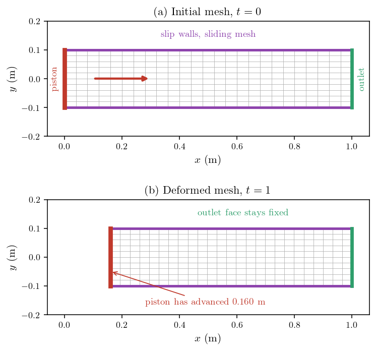
Figure 1: (a) The duct and its boundaries at rest. (b) The same mesh at $t=1$ s: the piston has advanced and the cells have compressed, while the outlet face has not moved.

Setting the ALE method up

The method is enabled in the GUI, together with the quantity that governs how the interior mesh absorbs the boundary motion:

<ale_method status="on">
  <mesh_viscosity type="isotrop"/>
  <formula>mesh_viscosity = 1;</formula>
</ale_method>

The mesh displacement is obtained by solving a diffusion equation whose "viscosity" is this field. Uniform viscosity spreads the deformation evenly, and that is what makes every cell of the duct share the compression equally, as measured below. Making the viscosity larger near a region you want to protect is how you keep good cells where they matter and push the distortion elsewhere.

The piston motion is a formula on its boundary:

<wall label="piston" field_id="none">
  <velocity_pressure choice="off"/>
  <ale choice="fixed_displacement">
    <formula>mesh_displacement[0] = 0.2*(t - 0.2*(1. - exp(-t/0.2)));
mesh_displacement[1] = 0.;
mesh_displacement[2] = 0.;</formula>
  </ale>
</wall>

The displacement is counted from the initial mesh, not from the previous time step, so the formula is the position law itself. The fluid velocity at the piston needs no separate treatment: it is a wall, and the ALE machinery gives it the velocity of the mesh.

The other boundaries decide whether anything moves

This is the trap worth remembering. Every boundary needs an ALE condition, and the natural-looking choice of holding them all in place makes the case do nothing at all: with fixed_boundary on the side walls, their nodes cannot translate in \(x\), and since they bracket the whole duct the mesh has nowhere to go. The piston pushes and the mesh stays put.

sliding_boundary is the right answer for a wall that must stay a wall while letting nodes travel along it. Only the outlet, which really should not move, is fixed.

Prescribed displacement, not prescribed velocity

The GUI also offers fixed_velocity, which reads more naturally for a piston. With the legacy ALE solver it does nothing: in cs_gui_mobile_mesh.cpp the routine that handles it evaluates the formula, writes the result into a local array, marks the faces, and frees the array without ever using the values, leaving a comment that they are handled elsewhere. Nothing else picks them up. The mesh never moves, and no warning is issued.

The symptom is worth knowing because it is confusing: the fluid velocity comes out correct anyway, since a fixed wall with an imposed normal velocity injects the same flow rate. Only the mesh betrays the problem. Prescribing the displacement, as above, works.

Seeing the mesh move

One last detail, this one merely cosmetic. Post-processing writers default to a fixed mesh, so the output holds the initial geometry no matter how much the mesh has moved. Ask for moving coordinates:

<time_dependency choice="transient_coordinates"/>

Numerical setup

Setting	Value
Mesh	\(100\times20\times1\) cells
Time step	0.002 s (constant)
Iterations	500 (final time 1 s)
Velocity-pressure algorithm	SIMPLEC
Mesh viscosity	isotropic, uniform

Running the simulation

cd CASE
code_saturne run

The run takes under two minutes on one core.

Results and verification

Everything is compared with the closed-form solution above. The piston travels 16 percent of the duct length, so the cells at the piston end lose about a sixth of their length by the end of the run.

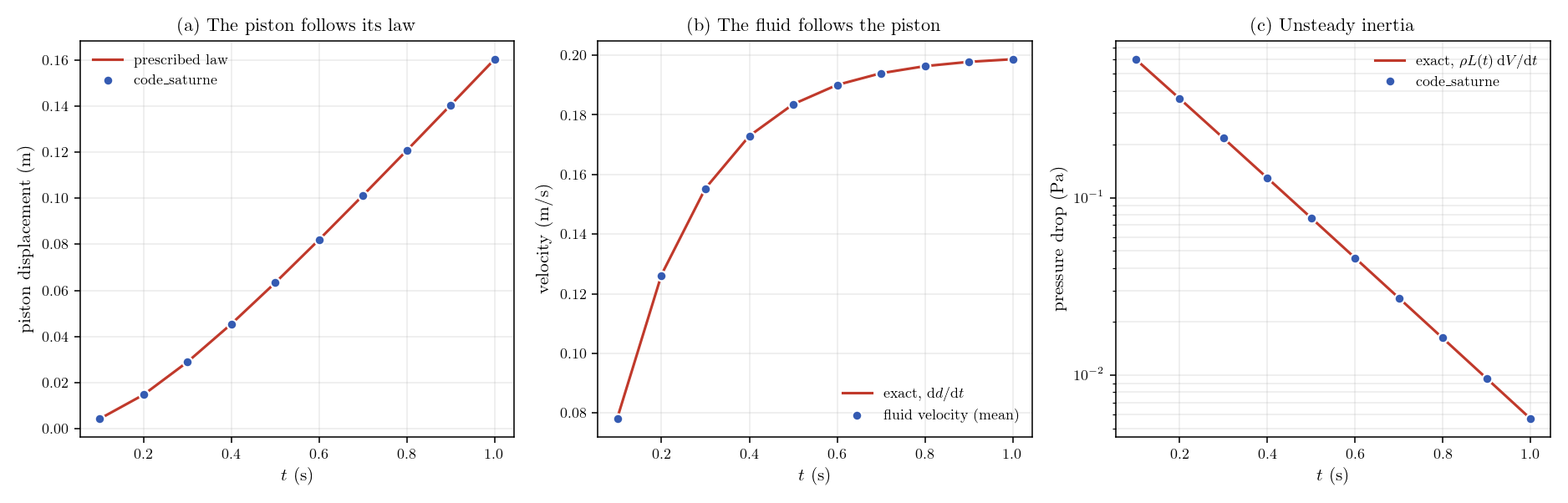
Figure 2: The three exact checks. Lines are the closed-form solution, markers the computation.

Quantity at \(t=1\) s	Computed	Exact
Piston displacement (m)	0.16027	0.16027
Fluid velocity (m/s)	0.19865	0.19865
Velocity spread across the domain	\(5\times10^{-5}\)	0
Pressure drop (Pa)	\(5.68\times10^{-3}\)	\(5.66\times10^{-3}\)

The piston lands on its prescribed law, and the fluid velocity on the derivative of that law, to the printing precision. The velocity is uniform across the whole domain to a few \(10^{-5}\), which is the real content of the mass-conservation check on a shrinking domain: nothing is created or lost by the moving cells.

The pressure drop is the most demanding of the three, because it tests the unsteady term rather than the kinematics, and because it decays by two orders of magnitude over the run as the piston stops accelerating. The computation follows it throughout.

Watching the mesh move

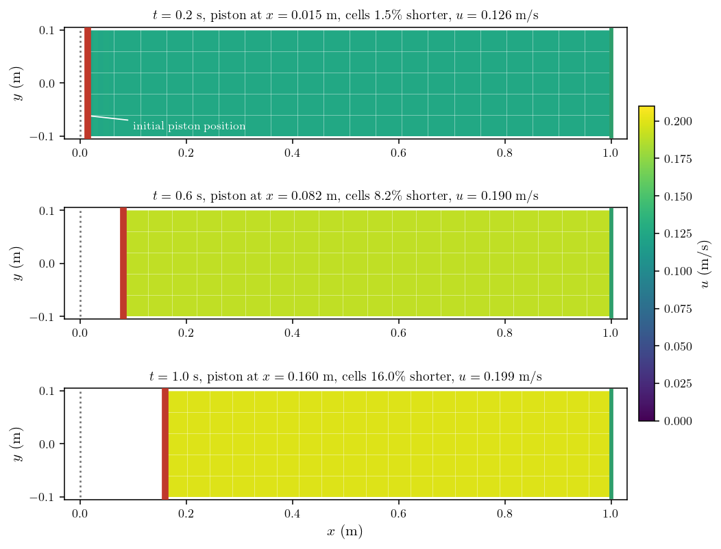
Figure 3: Three instants of the computation. The piston advances, the domain shortens, and the colour shows the fluid accelerating with it. The dotted line marks where the piston started.

Two things are worth reading off this figure. The cells compress by the same fraction everywhere, 16 percent by the end, rather than the ones next to the piston absorbing the whole stroke: that even sharing is what a uniform mesh viscosity buys, and measuring it against the linear law gives a maximum departure of \(1.5\times10^{-5}\) m. And the colour is flat across each panel, which is the one-dimensional solution holding as the mesh deforms.

If the deformation had to be kept away from a sensitive region, a larger mesh viscosity there would push the distortion elsewhere. That is the knob to reach for when a moving boundary starts to spoil cells that matter.

Summary

ALE turns a moving boundary into a moving mesh, and in code_saturne it needs no user routine: the motion is a formula on the boundary and the method is a switch in the GUI. Two settings decide whether it works. The other boundaries must be allowed to move, so walls that the mesh has to slide along are sliding rather than fixed, and the motion must be prescribed as a displacement, since the prescribed-velocity option is accepted by the interface and dropped by the legacy solver without warning.

Verified against the exact one-dimensional solution, the result is as good as the statement of the problem: the boundary follows its law, the fluid follows the boundary, mass is conserved on cells that are shrinking as they are integrated, and the unsteady pressure drop is right over two decades of decay.

One practical caveat that this case avoids by construction: the piston here only ever pushes. Reversing it makes the outlet an inlet for part of the cycle, and a standard outlet condition handles that badly, which shows up as velocities several times the piston speed. Oscillating boundaries need a boundary condition that tolerates inflow, not a plain outlet.

References

1. code_saturne documentation: https://code-saturne.org/doc/.
2. J. Donea, A. Huerta, J.-P. Ponthot, A. Rodriguez-Ferran, "Arbitrary Lagrangian-Eulerian Methods", in Encyclopedia of Computational Mechanics, Wiley, 2004.

Authors

Simvia - Questions, remarks and requests are welcome.