1D Wall Thermal Response (Quench of a Heated Channel)

Browse this case on GitHub

A step-by-step tutorial for the 1D wall thermal module of code_saturne: the transient conduction across a solid wall is solved on an embedded 1D mesh, coupled to the flow at the fluid-side face, without meshing the solid. A hot laminar channel is quenched when the exterior of its bottom wall is suddenly exposed to a cold environment, and the coupled wall temperature is verified against the exact analytic solution of the 1D slab.

This module is the lightweight counterpart of conjugate heat transfer: where Th_Conjugate_Heat_Transfer meshes the solid and couples volume zones, the 1D wall module only needs boundary faces and a wall description (thickness, conductivity, capacity).

Maintained by Simvia, part of the tutoriel-code_saturne collection.

Learning objectives

After completing this tutorial you will be able to:

1. Activate the 1D wall thermal module (a routine-only feature, with no GUI path).
2. Select the coupled boundary faces and build the embedded 1D meshes across the wall thickness.
3. Prescribe the wall properties and the exterior boundary condition (Dirichlet with exchange coefficient) at every time step.
4. Run a true transient thermal calculation and monitor the coupled wall temperature.
5. Verify the coupled response against the exact analytic solution of a 1D slab.

Prerequisites

Requirement	Detail
code_saturne	v9.1
Background	Basic notions of transient heat conduction and convective heat transfer

If code_saturne is not yet installed, build it from the official homepage, pull a ready-to-use Singularity image from the Open Simulation Center, or pull the Simvia Docker image before continuing.

Case files

Th_1D_Wall_Thermal/
├── CASE/
│   ├── DATA/
│   │   └── setup.xml                    # pre-configured GUI case
│   └── SRC/
│       └── cs_user_1d_wall_thermal.cpp  # the showcased feature
├── FIGURES/                             # figures used in this README
└── README.md

There is no mesh file: the channel grid is built by code_saturne's internal Cartesian mesher, directly from setup.xml.

Physical model

The flow is laminar, incompressible and truly transient (physical time). The fluid enters hot and in thermal equilibrium with the wall; the transient is driven entirely by the wall quench. The temperature is a passive scalar:

\[ \rho c_p\left(\frac{\partial T}{\partial t}+\mathbf{u}\cdot\nabla T\right) =\nabla\cdot(k_f\nabla T). \]

Inside the bottom wall, the module solves the 1D transient conduction equation across the thickness on its own embedded mesh:

\[ \rho_s c_{p,s}\frac{\partial T}{\partial t} =\lambda_s\frac{\partial^2 T}{\partial x_n^2}, \qquad 0\le x_n\le e, \]

coupled to the fluid at \(x_n=0\) (the wall face temperature seen by the flow) and exposed at \(x_n=e\) to a cold exterior through an exchange coefficient:

\[ -\lambda_s\frac{\partial T}{\partial x_n}\Big|_{x_n=e} =h_{\mathrm{ext}}\left(T-T_{\mathrm{ext}}\right). \]

At \(t=0\) the whole system (fluid and wall) is at \(T_0\) and the cold exterior is switched on: the wall quenches, and its fluid-side temperature relaxes toward the steady balance between interior convection, wall conduction and exterior convection.

Flow parameters

Parameter	Value	Unit	Source
Inlet velocity \(U\)	0.5	\(\mathrm{m\,s^{-1}}\)	setup.xml: inlet/velocity_pressure/norm
Inlet and initial temperature \(T_0\)	340	K	setup.xml: inlet thermal dirichlet
Density \(\rho\)	1.2	\(\mathrm{kg\,m^{-3}}\)	setup.xml: density
Dynamic viscosity \(\mu\)	\(1.8\times10^{-5}\)	\(\mathrm{Pa\,s}\)	setup.xml: molecular_viscosity
Specific heat \(c_p\)	1005	\(\mathrm{J\,kg^{-1}\,K^{-1}}\)	setup.xml: specific_heat
Fluid conductivity \(k_f\)	0.025	\(\mathrm{W\,m^{-1}\,K^{-1}}\)	setup.xml: thermal_conductivity

With the channel height \(H=0.02\ \mathrm{m}\) (\(D_h=2H\)), the Reynolds number is \(Re_{D_h}=\rho U D_h/\mu\approx1330\) (laminar) and \(Pr\approx0.72\).

Wall parameters (the 1D module)

Parameter	Value	Unit	Source
Thickness \(e\)	5	mm	cs_user_1d_wall_thermal.cpp
Conductivity \(\lambda_s\)	0.03	\(\mathrm{W\,m^{-1}\,K^{-1}}\)	cs_user_1d_wall_thermal.cpp
Capacity \(\rho_s c_{p,s}\)	\(4.2\times10^{4}\)	\(\mathrm{J\,m^{-3}\,K^{-1}}\)	cs_user_1d_wall_thermal.cpp
Points across the thickness	20 (grading 1.1)	-	cs_user_1d_wall_thermal.cpp
Exterior temperature \(T_{\mathrm{ext}}\)	290	K	cs_user_1d_wall_thermal.cpp
Exterior coefficient \(h_{\mathrm{ext}}\)	50	\(\mathrm{W\,m^{-2}\,K^{-1}}\)	cs_user_1d_wall_thermal.cpp

The wall diffusivity \(\alpha_s=\lambda_s/(\rho_s c_{p,s})\approx7.1\times10^{-7}\ \mathrm{m^2\,s^{-1}}\) gives a conduction time \(e^2/\alpha_s\approx35\ \mathrm{s}\): the 80 s simulated reach the steady plateau.

Geometry and boundary conditions

The domain is a plane channel of length \(L=0.5\ \mathrm{m}\) and height \(H=0.02\ \mathrm{m}\), one cell thick in \(z\). The grid (100 x 40 cells) is built by the internal Cartesian mesher and refined geometrically toward the bottom wall.

Boundary	Type	Condition
inlet (\(x=0\))	Inlet	\(U=0.5\ \mathrm{m\,s^{-1}}\), \(T_0=340\ \mathrm{K}\)
outlet (\(x=L\))	Outlet	Standard outlet
bottom_wall (\(y=0\))	Wall	No slip; thermal BC replaced by the 1D wall module
top_wall (\(y=H\))	Wall	No slip, adiabatic
front / back	Symmetry	Quasi-2D

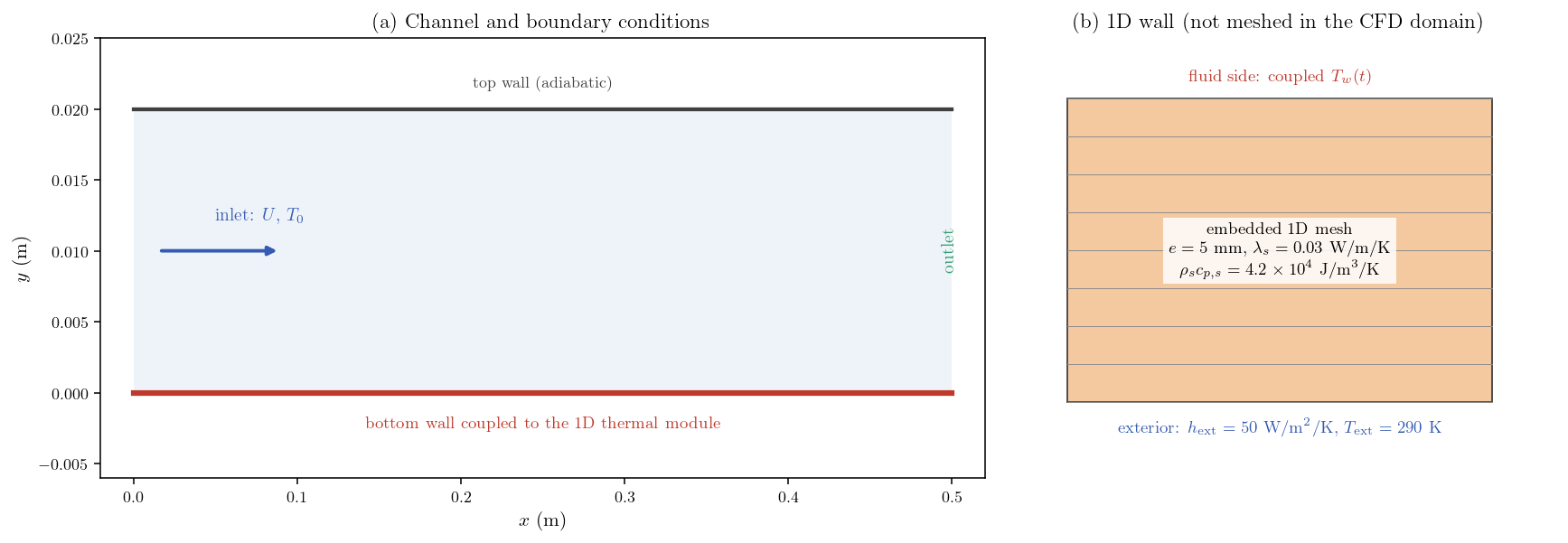
Figure 1: (a) Channel and boundary conditions. (b) The 1D wall attached to the bottom boundary: it exists only as an embedded 1D conduction mesh, not in the CFD domain.

The user routine (the feature)

The module has no GUI path: it activates when CASE/SRC/cs_user_1d_wall_thermal.cpp declares a positive number of coupled faces. The routine is called with three purposes:

1. Call 1: count the coupled faces. Here the bottom_wall GUI zone is retrieved with cs_boundary_zone_by_name and its face count sets nfpt1d (a positive value activates the module).
2. Call 2: list the faces (ifpt1d, in increasing order) and build each embedded 1D mesh: nppt1d points, thickness eppt1d, grading rgpt1d (refined on the fluid side), initial temperature tppt1d.
3. Call 3 (every time step): set the exterior boundary condition (iclt1d = 1: Dirichlet with exchange coefficient, tept1d, hept1d) and the wall properties (xlmbt1, rcpt1d), and advance the 1D solve with the local fluid time step (dtpt1d).

On the fluid side, the module then imposes the computed wall face temperature as the thermal boundary condition: no thermal wall setting is needed in the GUI for bottom_wall.

Numerical setup

Setting	Value
Time scheme	True transient, fixed \(\Delta t=0.01\ \mathrm{s}\)
Time steps	8000 (80 s)
Velocity-pressure algorithm	SIMPLEC
Turbulence	Off (laminar)
Gravity	Off

Running the simulation

From the tutorial directory:

Option A: Graphical interface

code_saturne gui CASE/DATA/setup.xml &

Review the setup, then launch with the Run button. The user routine in CASE/SRC/ is compiled automatically.

Option B: Command line

cd CASE
code_saturne run              # serial
code_saturne run --n 4        # parallel (4 MPI ranks)

Each run creates a time-stamped CASE/RESU/<id>/ containing run_solver.log, monitoring/ (probe CSV) and postprocessing/ (EnSight fields, including the boundary temperature used below).

Results and verification

Fluid response

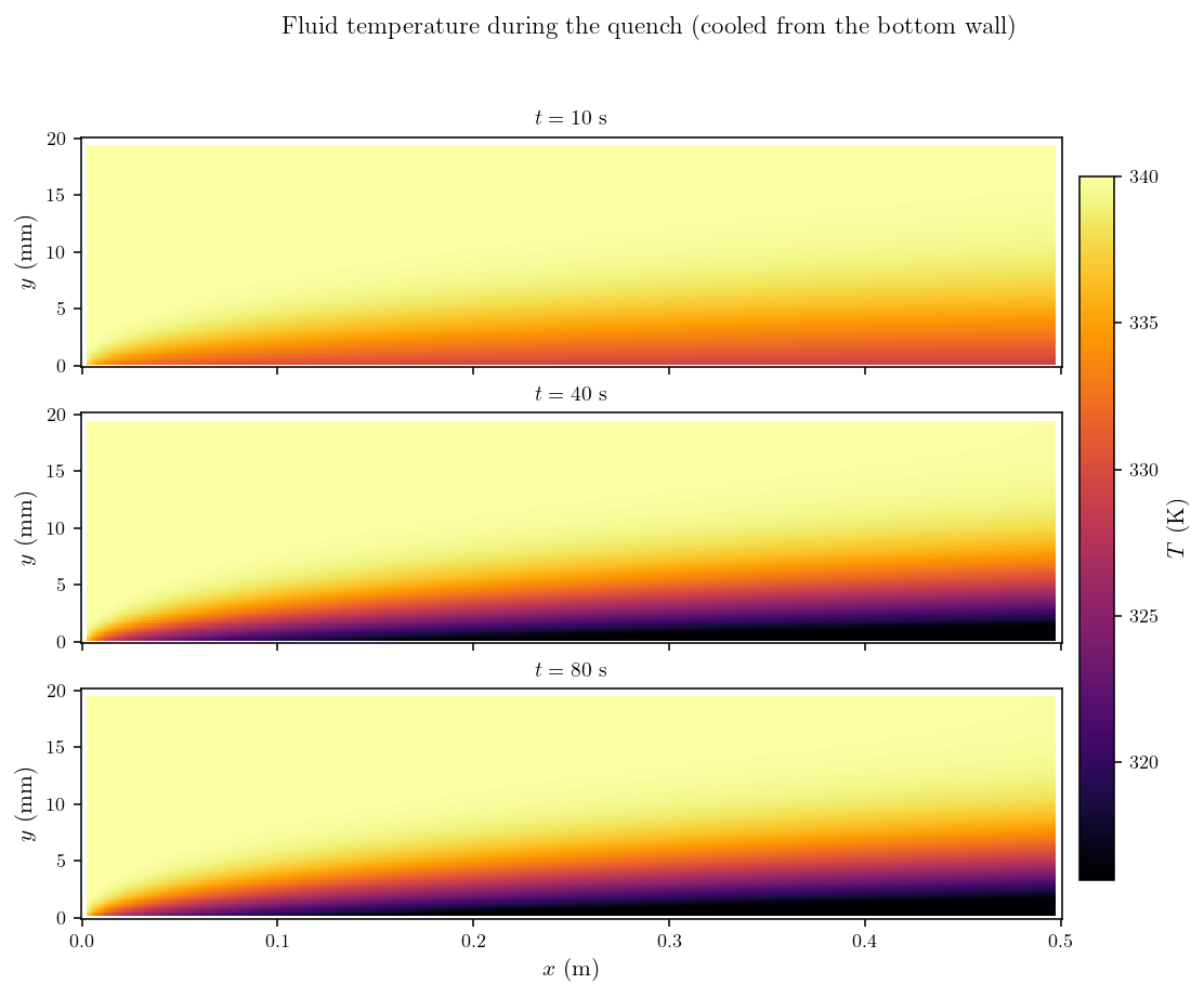
Figure 2: Fluid temperature during the quench. A cold thermal boundary layer grows from the bottom wall and thickens downstream while the wall temperature drops.

Wall temperature vs the exact 1D solution

The coupled wall temperature (averaged on the bottom wall around mid-channel, \(0.2<x<0.3\ \mathrm{m}\)) is compared with the exact analytic solution of the 1D slab with convection on both faces: interior fluid at \(T_0\) with the exchange coefficient measured from the run (\(h_{\mathrm{int}}\approx4.4\ \mathrm{W\,m^{-2}\,K^{-1}}\), close to the laminar correlation value \(Nu_{D_h}=7.54\), i.e. \(4.7\ \mathrm{W\,m^{-2}\,K^{-1}}\)), exterior at \(T_{\mathrm{ext}}\) with \(h_{\mathrm{ext}}\). The solution is the classical eigenfunction series, and its \(t\to\infty\) limit is the plateau given by the series thermal resistances \(1/h_{\mathrm{int}}+e/\lambda_s+1/h_{\mathrm{ext}}\).

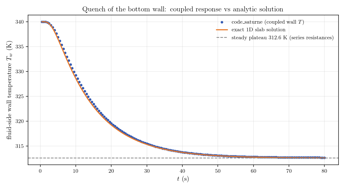
Figure 3: Quench of the bottom wall. The coupled code_saturne response follows the exact slab solution within 0.6 K and settles on the series-resistance plateau.

Quantity	code_saturne	Analytic
Wall temperature history (0 to 80 s)	-	max deviation 0.6 K, mean 0.2 K
Steady plateau	312.7 K	312.6 K

The agreement is within 0.6 K over a 27 K quench (about 2 percent of the transient amplitude); the residual deviation comes mainly from the slow axial growth of the thermal boundary layer, which the 1D model represents through a single constant \(h_{\mathrm{int}}\).

Summary

This tutorial activated the 1D wall thermal module of code_saturne on the bottom wall of a hot laminar channel and quenched it through a cold exterior condition. The feature is entirely driven by one user routine (face selection, embedded 1D meshes, per-step exterior condition), since it has no GUI path, and couples back to the flow through the wall face temperature. The computed response matches the exact 1D slab solution within 0.6 K up to the series-resistance plateau. The module is the light alternative to conjugate heat transfer whenever the wall can be treated as locally one-dimensional; for meshed solids and multidimensional conduction, see the internal-coupling tutorial Th_Conjugate_Heat_Transfer.

References

1. code_saturne documentation: https://code-saturne.org/doc/.
2. H. S. Carslaw and J. C. Jaeger, Conduction of Heat in Solids, 2nd ed., Oxford University Press, 1959.
3. F. P. Incropera, D. P. DeWitt, T. L. Bergman, and A. S. Lavine, Fundamentals of Heat and Mass Transfer, Wiley.

Authors

Simvia - Questions, remarks and requests are welcome.