Mapped Inlet (Recycling a Downstream Profile)

Browse this case on GitHub

Turbulent studies almost always need a fully developed profile at the inlet, and there is no cheap way to write one down. An analytical log-law profile never quite matches the mesh and the turbulence model you actually use, so the flow spends the first part of your domain readjusting. Meshing a long upstream development section works, but you pay for cells that carry no result.

Recycling sidesteps the problem. Instead of prescribing the inlet, you copy it from a plane a few channel heights downstream, at every time step. The flow feeds itself, and what it converges to is the profile that this mesh and this turbulence model produce on their own.

This tutorial does that on a turbulent channel and measures what it is worth. On a domain ten half-heights long the profile is developed from the first cell, and it reproduces the independent periodic-channel computation of Inc_Turbulent_Channel. The same domain fed with a uniform inlet is still 3 percent away from that profile at its outlet.

Maintained by Simvia, part of the tutoriel-code_saturne collection.

Learning objectives

After completing this tutorial you will be able to:

1. Build the locator that links every inlet face to the cell found a prescribed distance downstream (cs_boundary_conditions_map).
2. Copy the downstream values onto the inlet at every time step, rescaled so that the mass flow rate imposed in the GUI is preserved (cs_boundary_conditions_mapped_set).
3. Check that the resulting inlet is fully developed, by comparing profiles along the channel, against a periodic-channel computation, and against the law of the wall.

Prerequisites

Requirement	Detail
code_saturne	v9.1
Tutorials	Inc_Turbulent_Channel (the periodic channel used here as reference)
Background	Wall-bounded turbulence and the law of the wall

If code_saturne is not yet installed, build it from the official homepage, pull a ready-to-use Singularity image from the Open Simulation Center, or pull the Simvia Docker image before continuing.

Case files

Inc_Mapped_Inlet/
├── CASE/
│   ├── DATA/
│   │   └── setup.xml                        # pre-configured GUI case
│   └── SRC/
│       └── cs_user_boundary_conditions.cpp  # the showcased feature
├── FIGURES/                                 # figures used in this README
└── README.md

The channel is built by the internal Cartesian mesher from setup.xml, so there is no mesh file to ship.

Physical model

The flow is incompressible, statistically steady and fully turbulent between two parallel walls a distance \(2h\) apart, closed with the k-\(\omega\) SST model integrated down to the wall rather than through a wall function.

The channel is the one of the periodic tutorial, in the same non-dimensional form, which is what makes the two computations directly comparable.

Parameter	Value	Source
Density \(\rho\)	1	setup.xml: density
Dynamic viscosity \(\mu\)	\(2.5316\times10^{-3}\) (\(=1/395\))	setup.xml: molecular_viscosity
Half-height \(h\)	1	mesh
Imposed bulk velocity \(U_b\)	16.9	setup.xml: inlet/velocity_pressure/norm

The bulk velocity is the one the periodic computation settles at, so both cases carry the same mass flow rate; the bulk Reynolds number is \(Re_b=\rho\,U_b\,2h/\mu\simeq1.34\times10^{4}\).

Geometry and boundary conditions

The domain is a plane channel \(10h\) long and \(2h\) high, one cell thick in \(z\), meshed with \(100\times150\) cells. The wall-normal spacing follows a parabolic law that puts the first cell centre at \(y^+\simeq0.4\), inside the viscous sublayer.

Boundary	Type	Condition
inlet (\(x=0\))	Inlet	flow rate from setup.xml, profile recycled from \(x=5h\)
outlet (\(x=10h\))	Outlet	Standard outlet
walls (\(y=\pm h\))	Wall	No slip
sym (\(z\) planes)	Symmetry	Quasi-2D

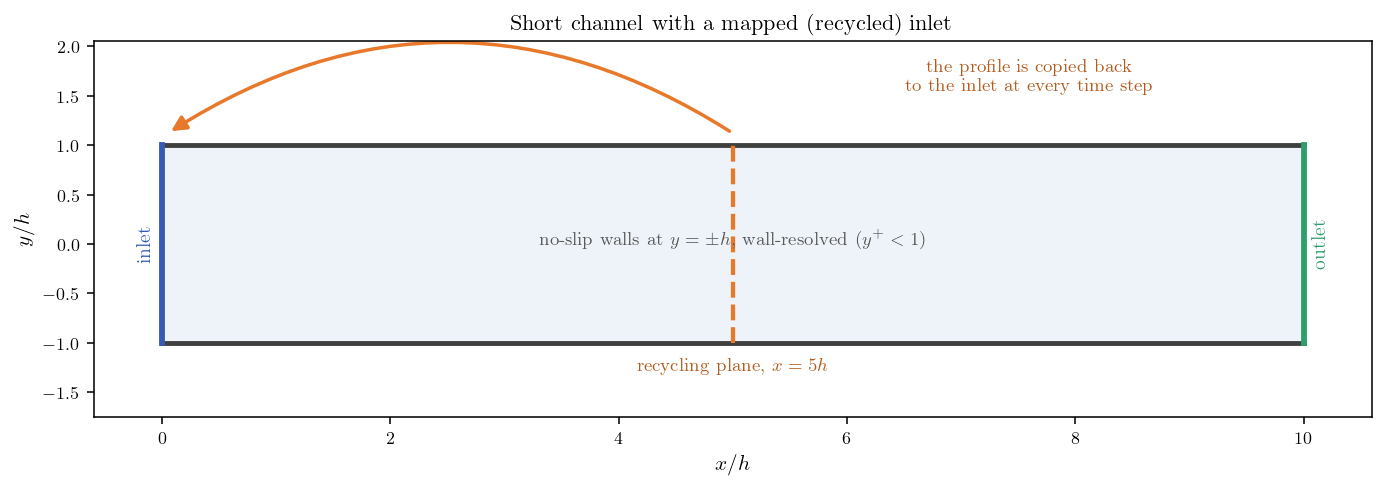
Figure 1: The short channel. At every time step the values found on the recycling plane ($x=5h$) are copied onto the inlet.

The mapped inlet

Everything is in CASE/SRC/cs_user_boundary_conditions.cpp, and it comes down to two calls.

At the first time step, a locator associates every inlet face with the cell that contains the point (face centre + shift). The shift is the recycling length:

cs_real_3_t coord_shift[1] = {{5.0, 0., 0.}};

_inlet_locator = cs_boundary_conditions_map(CS_MESH_LOCATION_CELLS,
                                            n_cells, zn->n_elts,
                                            cells_ids, zn->elt_ids,
                                            coord_shift,
                                            0,       /* uniform shift */
                                            0.10);   /* location tolerance */

The locator is stored in a static variable: building it involves a geometric search, so it is done once and reused, not rebuilt at every step.

From the second step on, the values found there are copied onto the inlet, field by field:

const int normalize = (f == CS_F_(vel)) ? 1 : 0;

cs_boundary_conditions_mapped_set(f, _inlet_locator, CS_MESH_LOCATION_CELLS,
                                  normalize, 0,
                                  zn->n_elts, zn->elt_ids, nullptr);

Why this converges

Nothing here imposes a developed profile; the loop finds it. The inlet at step \(n\) is the interior solution at step \(n-1\), so at convergence the inlet profile is equal to the profile at \(x=5h\). A flow whose profile is the same at \(x=0\) and at \(x=5h\) is, by definition, invariant in the streamwise direction, which is what "fully developed" means. The developed profile is the fixed point of the recycling loop, and the calculation walks to it on its own.

The two choices that matter

normalize = 1 on the velocity is not a detail. The copied profile is rescaled so that its surface integral matches the one prescribed in the GUI: the mapping sets the shape of the profile and you keep control of the mass flow rate. Without it, nothing pins the flow rate and it drifts with the loop. The turbulence variables have no such constraint and are copied as they are (normalize = 0).

The recycling length is the second choice. It must be long enough that the plane you sample has forgotten the inlet: sampling too close means copying back your own boundary condition, which is degenerate. It also has to stay well inside the domain, since the shifted point must land in a real cell. Five half-heights is comfortable here, and the verification below shows the loop does its job.

One consequence surprises people: the inlet velocity and turbulence set in the GUI only serve the very first time step. Refining them is wasted effort, since the mapping overwrites them from step two onwards.

Numerical setup

Setting	Value
Turbulence model	k-\(\omega\) SST, wall-resolved
Steady strategy	Local (pseudo) time-stepping
Iterations	4000
Velocity-pressure algorithm	SIMPLEC
Recycling length	\(5h\) (_recycling_length in the routine)

Running the simulation

From the tutorial directory:

cd CASE
code_saturne run              # serial
code_saturne run --n 4        # parallel (4 MPI ranks)

The user routine is compiled automatically. To reproduce the comparison below, run the case a second time with CASE/SRC/ emptied: the inlet then keeps the uniform profile of the GUI, and you get the developing-flow reference.

Results and verification

Three checks, from the weakest to the strongest. Streamwise invariance is necessary but not sufficient, since a wrong profile could also be invariant. Agreement with an independent computation of the same channel is the real test. The law of the wall and the friction then confirm the physics.

Streamwise invariance

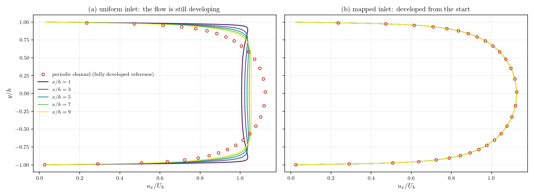
Figure 2: Streamwise velocity at $x/h=1,3,5,7,9$ (lines), with the periodic-channel profile as circles. With a uniform inlet (a) the profiles change all along the channel and none reaches the reference. With the mapped inlet (b) the five stations are indistinguishable and pass through the reference points.

Quantity	Mapped inlet	Uniform inlet
Profile change between \(x=1h\) and \(x=9h\)	0.00 % of \(U_b\)	30.6 % of \(U_b\)
Profile change between \(x=7h\) and \(x=9h\)	0.00 % of \(U_b\)	3.0 % of \(U_b\)
Deviation from the periodic reference at \(x=9h\)	0.03 % max, 0.01 % mean	9.8 % max, 5.7 % mean
Friction velocity \(u_\tau\) at \(x=9h\)	0.973	1.026

The recycled case is invariant to the printing precision, and its profile is the periodic one. The uniform case tells the other half of the story: ten half-heights are not enough to develop a channel from a flat profile, and the error it makes is not only on the profile shape. Its wall friction is 5 percent too high, because a thin boundary layer shears harder than a developed one.

Wall friction

Measured the same way on both, the friction velocity of the recycled case and of the periodic computation agree to 0.03 percent, which gives \(Re_\tau=384\). Since agreeing with another computation only proves consistency, the Dean (1978) correlation for plane channels, \(c_f=0.073\,Re_b^{-0.25}\), provides an external reference: it sits 1.2 percent above the computed friction.

Law of the wall

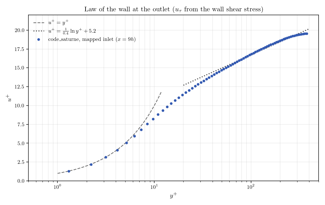
Figure 3: Outlet profile in wall units, with $u_\tau$ from the wall shear stress written by the solver. The near-wall points follow $u^+=y^+$ and the outer points the logarithmic law.

The profile follows \(u^+=y^+\) through the viscous sublayer, then the logarithmic law \(u^+=\frac{1}{0.4}\ln y^+ + 5.2\) across the log layer: the boundary layer delivered by the recycled inlet is the one expected of a wall-resolved channel.

Summary

A mapped inlet buys a fully developed turbulent inflow for the price of a short recycling section. Two calls do the work: cs_boundary_conditions_map builds, once, the locator that ties each inlet face to a cell \(5h\) downstream, and cs_boundary_conditions_mapped_set copies the values there at every time step, rescaled so the imposed mass flow rate is preserved. The loop converges to the profile that is invariant in \(x\), which is the developed one: here it reproduces an independent periodic-channel computation, both on the velocity profile and on the wall friction, agrees with the Dean friction correlation, and recovers the law of the wall. The same domain with a uniform inlet is still developing at its outlet.

The profile obtained this way is developed for the geometry that produces it, which is exactly why it is consistent with your mesh and your turbulence model, and also why it cannot represent an inflow whose upstream history is genuinely different. In unsteady computations, keep in mind that recycling also feeds the turbulent structures back to the inlet, which can lock the solution onto the travel time of the recycling section.

References

1. code_saturne documentation: https://code-saturne.org/doc/.
2. R. B. Dean, "Reynolds number dependence of skin friction and other bulk flow variables in two-dimensional rectangular duct flow", Journal of Fluids Engineering, vol. 100, pp. 215-223, 1978.
3. S. B. Pope, Turbulent Flows, Cambridge University Press, 2000.

Authors

Simvia - Questions, remarks and requests are welcome.