Turbulent Backward-Facing Step (Driver-Seegmiller)
A step-by-step tutorial for simulating the incompressible turbulent flow over a backward-facing step with code_saturne, using the \(k\)-\(\omega\) SST RANS model. The sudden expansion separates the boundary layer at the step edge and produces a recirculation bubble that reattaches downstream. The reattachment length is verified against the Driver & Seegmiller (1985) experiment, also distributed as a NASA Turbulence Modeling Resource validation case.
Maintained by Simvia, part of the tutoriel-code_saturne collection.
Learning objectives
After completing this tutorial you will be able to:
- Set up an incompressible, steady RANS simulation of a separated internal flow in code_saturne.
- Configure the \(k\)-\(\omega\) SST turbulence model with consistent inlet values.
- Apply inlet / outlet / no-slip wall / symmetry boundary conditions on a wall-refined mesh.
- Drive a steady solution with local (pseudo) time-stepping and the SIMPLEC coupling.
- Extract the wall skin-friction coefficient and verify the reattachment length against experiment.
Prerequisites
| Requirement | Detail |
|---|---|
| code_saturne | v9.1 |
| Background | Basic notions of RANS turbulence modelling, boundary-layer separation and reattachment |
If code_saturne is not yet installed, build it from the official homepage, pull a ready-to-use Singularity image from the Open Simulation Center, or pull the Simvia Docker image before continuing.
Case files
Inc_Turbulent_Step/
├── CASE/
│   └── DATA/
│       └── setup.xml          # pre-configured GUI case
├── MESH/
│   └── backwardFacingStep.med # wall-refined hexahedral mesh
├── FIGURES/                   # figures used in this README
└── README.md
Physical model
The flow is steady, incompressible and fully turbulent, governed by the Reynolds-Averaged Navier-Stokes (RANS) equations closed with the two-equation \(k\)-\(\omega\) SST model:
The SST model blends a near-wall \(k\)-\(\omega\) formulation with a \(k\)-\(\varepsilon\) behaviour in the free stream and is a standard choice for adverse-pressure-gradient and separated flows such as this one. The flow is isothermal, single-phase and gravity is neglected.
Flow parameters
| Quantity | Symbol | Value | Source in setup.xml |
|---|---|---|---|
| Density | \(\rho\) | \(1\ \mathrm{kg\,m^{-3}}\) | physical_properties/.../density |
| Dynamic viscosity | \(\mu\) | \(1.56\times10^{-5}\ \mathrm{Pa\,s}\) | molecular_viscosity |
| Kinematic viscosity | \(\nu=\mu/\rho\) | \(1.56\times10^{-5}\ \mathrm{m^2\,s^{-1}}\) | derived |
| Inlet velocity | \(U_{\mathrm{ref}}\) | \(44.2\ \mathrm{m\,s^{-1}}\) | inlet/velocity_pressure/norm |
| Step height | \(h\) | \(0.0127\ \mathrm{m}\) | (geometry) |
| Inlet \(k\) | \(k_\infty\) | \(1.0904\times10^{-3}\ \mathrm{m^2\,s^{-2}}\) | inlet/turbulence/formula |
| Inlet \(\omega\) | \(\omega_\infty\) | \(7766.6\ \mathrm{s^{-1}}\) | inlet/turbulence/formula |
| Reference pressure | \(p_{\mathrm{ref}}\) | \(101325\ \mathrm{Pa}\) | reference_pressure |
The Reynolds number based on the step height is
The inlet turbulence is set from a turbulence intensity \(I=0.061\%\) and a viscosity ratio \(\nu_t/\nu=0.009\), matching the reference free-stream conditions:
Geometry and boundary conditions
The step of height \(h\) is located at \(x=0\). Upstream, the lower wall sits at \(y=h\) so the incoming channel is \(8h\) tall; downstream it drops to \(y=0\), giving a \(9h\) channel and an expansion ratio of \(9/8=1.125\). The domain extends far enough upstream and downstream to remove any influence of the inlet and outlet on the separated region.
| Direction | Extent | Normalized |
|---|---|---|
| Streamwise \(x\) | \(-1.651\) to \(0.635\ \mathrm{m}\) | \(-130h\) to \(50h\) |
| Vertical \(y\) | \(0\) to \(0.1143\ \mathrm{m}\) | \(0\) to \(9h\) |
| Spanwise \(z\) | \(0\) to \(0.0127\ \mathrm{m}\) | \(0\) to \(h\) (one cell) |
The no-slip walls begin about \(110h\) upstream of the step; the short sections between the inlet and the start of the walls are treated as symmetry so the uniform inlet stream enters cleanly before the boundary layers develop.
| Mesh group | code_saturne type | Physical role |
|---|---|---|
inlet |
Inlet | Uniform streamwise inflow \(U_{\mathrm{ref}}\), prescribed \(k,\omega\) |
outlet |
Outlet | Downstream flow exit |
lowerWall |
Wall | Lower no-slip wall and step surface |
upperWall |
Wall | Upper no-slip wall |
lowerWallStartup / upperWallStartup |
Symmetry | Short inlet-startup sections |
front / back |
Symmetry | Faces of the thin extrusion (2D formulation) |

Figure 1: Mid-span mesh and boundary-condition assignment. The mesh is
strongly refined toward the walls and around the step corner. The front and
back faces (normal to the spanwise direction) are symmetry boundaries and are
not visible in this $x$-$y$ slice.
The supplied hexahedral mesh (MESH/backwardFacingStep.med) has 20 540 cells
(41 746 boundary faces), one cell thick in \(z\), refined so that \(y^+\lesssim1\)
over most of the lower wall.
Numerical setup
| Setting | Value | Source in setup.xml |
|---|---|---|
| Flow model | Incompressible | velocity_pressure |
| Turbulence model | \(k\)-\(\omega\) SST | turbulence model="k-omega-SST" |
| Steady strategy | Local (pseudo) time-stepping | time_parameters/time_passing |
| Velocity-pressure coupling | SIMPLEC | velocity_pressure_algo |
| Pseudo-iterations | 2000 | time_parameters/iterations |
| Reference time step | \(10^{-4}\ \mathrm{s}\) | time_step_ref |
| Max Courant / Fourier | 1 / 10 | max_courant_num / max_fourier_num |
| Gravity | Disabled | gravity |
Because local time-stepping is used to reach a steady state, the reported "time" is a pseudo-time and does not represent a physical duration. The velocity and turbulence fields are initialized with the inlet values.
Running the simulation
From the tutorial directory:
Option A: Graphical interface
code_saturne gui CASE/DATA/setup.xml &
Review the pre-configured setup, then launch with the Run button. Set the number of processes under Calculation management > Performance settings for a parallel run.
Option B: Command line
cd CASE
code_saturne run              # serial
code_saturne run --n 4        # parallel (4 MPI ranks)
Each run creates a time-stamped CASE/RESU/<id>/ containing run_solver.log,
monitoring/ (probe CSV time series) and postprocessing/ (EnSight Gold volume
and boundary fields, including the wall boundary_stress used below).
Results and verification
Recirculation and reattachment
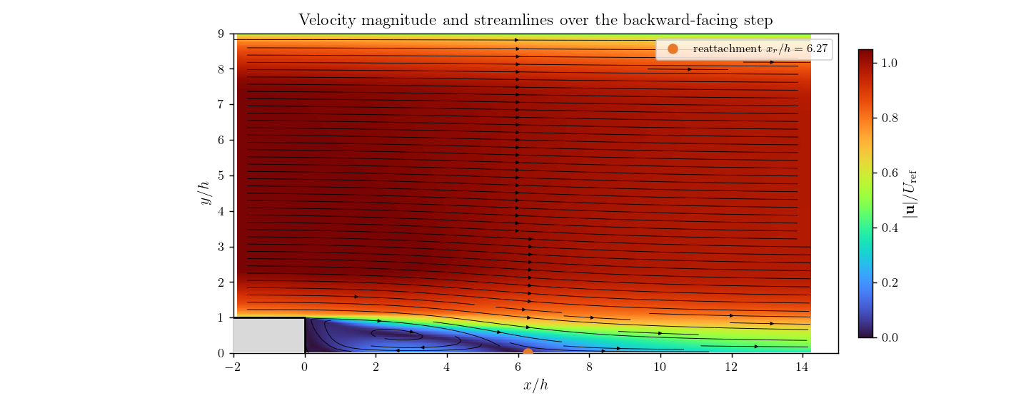
Figure 2: Velocity magnitude (normalized by $U_{\mathrm{ref}}$) and
streamlines near the step. The flow separates at the edge, a recirculation
bubble forms along the lower wall under a turbulent shear layer, and the mean
flow reattaches at $x_r/h=6.27$ (orange marker).
Skin friction and reattachment length
The mean reattachment point is where the lower-wall streamwise skin-friction coefficient changes sign from negative (reversed near-wall flow) to positive:
The wall shear is read directly from the boundary_stress field exported on
lowerWall.
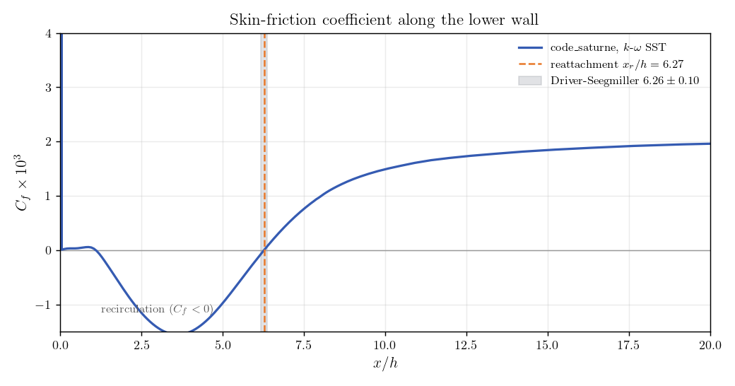
Figure 3: Lower-wall skin-friction coefficient. $C_f<0$ inside the
recirculation bubble; the first downstream zero-crossing gives the reattachment
length, which falls inside the experimental band.
| Quantity | code_saturne (\(k\)-\(\omega\) SST) | Reference |
|---|---|---|
| Reattachment length \(x_r/h\) | 6.27 | \(6.26\pm0.10\) (Driver & Seegmiller) |
| Lower-wall resolution \(y^+\) | \(\approx0.8\) mean (below 1 over most of the wall) | target \(\lesssim1\) |
The computed reattachment length agrees with the experiment to within its uncertainty. The near-wall mesh keeps \(y^+\) below one over most of the lower wall, so the boundary layer is wall-resolved (no wall functions); \(y^+\) rises to a few units only very locally near the sharp step corner, where the shear peaks.
Summary
This tutorial set up and verified a turbulent backward-facing step at \(Re_h=3.6\times10^4\) with the \(k\)-\(\omega\) SST model. The steady RANS solution reproduces the separation, recirculation and reattachment of the Driver-Seegmiller experiment, and the extracted reattachment length \(x_r/h=6.27\) matches the measured \(6.26\pm0.10\). The case is a compact, reproducible benchmark for separated-flow turbulence modelling and for extracting wall quantities from the boundary output.
Note that a single-cell spanwise extrusion models the flow as two-dimensional, the inlet is uniform rather than a measured boundary-layer profile, and a steady RANS model returns only the mean flow. These are standard simplifications for this verification exercise.
References
- D. M. Driver and H. L. Seegmiller, "Features of a Reattaching Turbulent Shear Layer in Divergent Channel Flow," AIAA Journal, vol. 23, no. 2, pp. 163-171, 1985.
- NASA Langley Turbulence Modeling Resource, 2D Backward-Facing Step: https://turbmodels.larc.nasa.gov/backstep_val.html
- F. R. Menter, "Two-equation eddy-viscosity turbulence models for engineering applications," AIAA Journal, vol. 32, no. 8, pp. 1598-1605, 1994.
- code_saturne documentation: https://code-saturne.org/doc/
Authors
Simvia - Questions, remarks and requests are welcome.