Time-Table Inlet (Transient Boundary Condition from a CSV File)

Browse this case on GitHub

A step-by-step tutorial for time tables in code_saturne: a boundary condition that follows a time scenario read from a CSV file. The inlet velocity of a laminar channel ramps between plateaus according to DATA/inlet_velocity.csv, entirely from the GUI (no user routine): the table is declared in the setup and used inside the boundary formula as inlet_law[velocity]. The response is verified against the table itself, the analytic Poiseuille solution, and the quasi-steady pressure-gradient model with its inertial correction.

Maintained by Simvia, part of the tutoriel-code_saturne collection.

Learning objectives

After completing this tutorial you will be able to:

1. Declare a time table from a CSV file in the GUI (name, delimiter, skipped header rows, column names).
2. Use the table inside any MEG formula with the table[column] syntax, interpolated at the current time.
3. Drive a transient inlet velocity through plateaus and ramps without writing code.
4. Check from the solver log (mass-flow budget) that the imposed inlet follows the table.
5. Verify the response against the Poiseuille solution and the quasi-steady pressure-gradient model.

Prerequisites

Requirement	Detail
code_saturne	v9.1
Background	Basic notions of laminar channel flow

If code_saturne is not yet installed, build it from the official homepage, pull a ready-to-use Singularity image from the Open Simulation Center, or pull the Simvia Docker image before continuing.

Case files

Inc_Time_Table_Inlet/
├── CASE/
│   └── DATA/
│       ├── setup.xml            # pre-configured GUI case
│       └── inlet_velocity.csv   # the time table (shipped with the case)
├── FIGURES/                     # figures used in this README
└── README.md

There is no mesh file: the channel grid is built by code_saturne's internal Cartesian mesher, directly from setup.xml.

Physical model

The flow is laminar, incompressible and truly transient. A viscous fluid enters a plane channel with a velocity that follows the time table; between the inlet transients, the flow relaxes to the steady plane Poiseuille solution

\[ u(y)=6\,U\,\frac{y}{H}\Big(1-\frac{y}{H}\Big), \qquad -\frac{\mathrm{d}p}{\mathrm{d}x}=\frac{12\,\mu\,U}{H^{2}}, \]

and during the ramps the established region follows the quasi-steady model augmented by the uniform inertial contribution:

\[ -\frac{\mathrm{d}p}{\mathrm{d}x} =\frac{12\,\mu\,U(t)}{H^{2}}+\rho\,\frac{\mathrm{d}U}{\mathrm{d}t}. \]

Flow parameters

Parameter	Value	Unit	Source
Density \(\rho\)	900	\(\mathrm{kg\,m^{-3}}\)	setup.xml: density
Dynamic viscosity \(\mu\)	0.09	\(\mathrm{Pa\,s}\)	setup.xml: molecular_viscosity
Inlet velocity \(U(t)\)	0.1 to 0.5	\(\mathrm{m\,s^{-1}}\)	DATA/inlet_velocity.csv
Reynolds number \(Re_{D_h}\)	40 to 200	-	derived (\(D_h=2H\))

The development length at the highest plateau is \(L_{\mathrm{dev}}\approx0.05\,Re_{D_h}\,D_h\approx0.4\ \mathrm{m}<L\): the outlet region is fully developed at every plateau.

The time table (the feature)

The scenario lives in a plain CSV file, DATA/inlet_velocity.csv:

time,velocity
0,0.1
5,0.1
10,0.5
15,0.5
20,0.25
30,0.25

It is declared in the GUI (Physical properties, Time tables), which stores in setup.xml:

<time_tables>
  <table id="0" name="inlet_law" file_name="inlet_velocity.csv" delimiter=",">
    <skip_rows>1</skip_rows>
    <headers_list>time,velocity</headers_list>
  </table>
</time_tables>

and used in the inlet velocity formula simply as:

u_norm = inlet_law[velocity];

At every time step, inlet_law[velocity] is interpolated linearly at the current physical time (first column = time). The same syntax works in any MEG formula (boundary conditions, source terms, properties). For sources that are not CSV files, the same tables can be created in C with cs_user_time_table.

Geometry and boundary conditions

Plane channel, \(L=1\ \mathrm{m}\), \(H=0.02\ \mathrm{m}\), one cell thick in \(z\); built-in Cartesian mesh of \(100\times40\) cells, refined toward both walls (parabolic law).

Boundary	Type	Condition
inlet (\(x=0\))	Inlet	\(U(t)\) from the time table
outlet (\(x=L\))	Outlet	Standard outlet
bottom_wall, top_wall	Wall	No slip
front / back	Symmetry	Quasi-2D

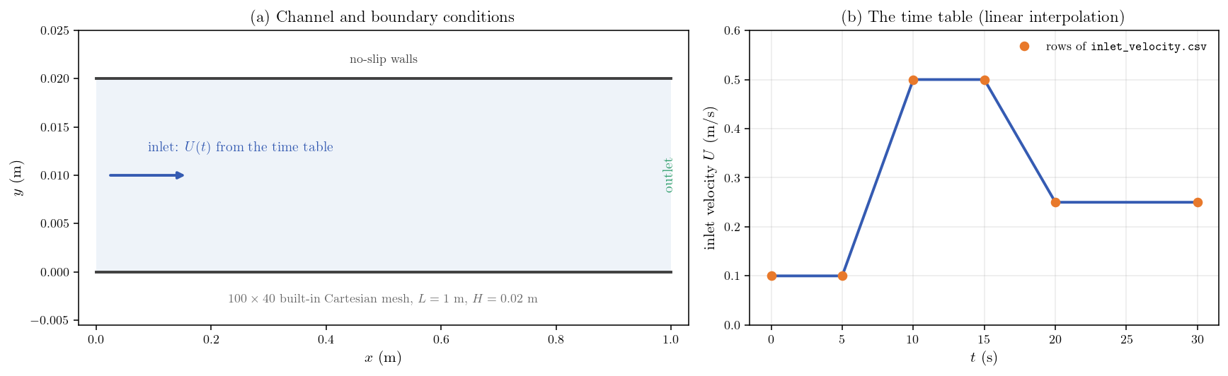
Figure 1: (a) Channel and boundary conditions. (b) The inlet scenario: plateaus at 0.1, 0.5 and 0.25 m/s connected by linear ramps, defined by the six rows of the CSV file.

Numerical setup

Setting	Value
Time scheme	True transient, fixed \(\Delta t=0.01\ \mathrm{s}\)
Time steps	3000 (30 s)
Velocity-pressure algorithm	SIMPLEC
Turbulence	Off (laminar)

Two probes record every time step: one at the inlet centreline, one at the outlet centreline (\(x=0.995\ \mathrm{m}\)).

Running the simulation

From the tutorial directory:

Option A: Graphical interface

code_saturne gui CASE/DATA/setup.xml &

The time table is visible under Physical properties, Time tables; the inlet formula under Boundary conditions. Launch with the Run button.

Option B: Command line

cd CASE
code_saturne run              # serial
code_saturne run --n 4        # parallel (4 MPI ranks)

The CSV file is staged automatically with the rest of DATA/. Each run creates a time-stamped CASE/RESU/<id>/ containing run_solver.log (including the boundary mass-flow budgets used below), monitoring/ and postprocessing/.

Results and verification

The inlet follows the table

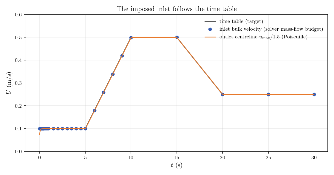
Figure 2: The inlet bulk velocity recovered from the solver mass-flow budget (dots) sits on the time table (line) through plateaus and ramps; the outlet centreline velocity divided by 1.5 (Poiseuille) follows the same scenario quasi-steadily.

The mass-flow budgets printed in run_solver.log give an inlet bulk velocity equal to the interpolated table within 0.16 percent of the maximum velocity (one time step of lag at the sampling instants). The outlet centreline velocity matches \(1.5\,U(t)\) with a mean deviation of 0.14 percent: the flow responds quasi-steadily at every point of the scenario.

Poiseuille profile and pressure gradient

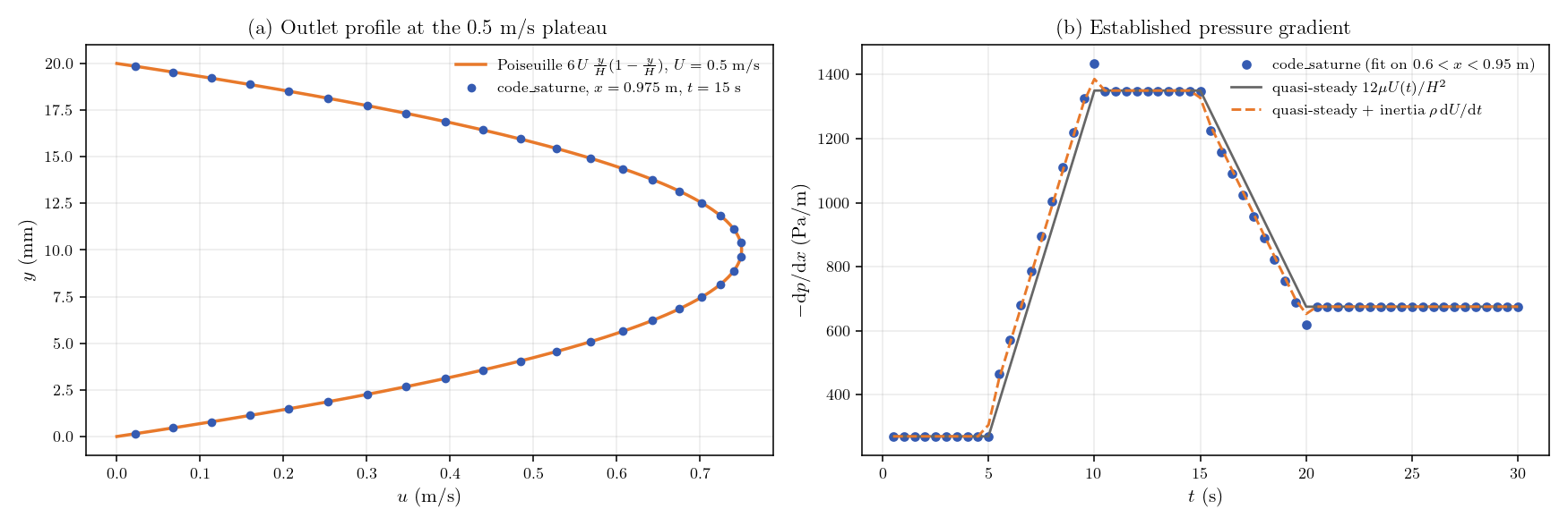
Figure 3: (a) Outlet profile at the 0.5 m/s plateau against the Poiseuille parabola. (b) Established pressure gradient (fit on $0.6

At the 0.5 m/s plateau, the established pressure gradient is \(1348\ \mathrm{Pa\,m^{-1}}\) against \(12\mu U/H^{2}=1350\ \mathrm{Pa\,m^{-1}}\) (0.2 percent). During the ramps the measured gradient follows the quasi-steady value shifted by \(\rho\,\mathrm{d}U/\mathrm{d}t\) (\(\pm\)72 and \(-45\ \mathrm{Pa\,m^{-1}}\) on the two ramps), the expected inertial cost of accelerating the whole channel.

Summary

This tutorial drove a transient inlet with a time table: a six-row CSV file declared in the GUI and used in the inlet formula as inlet_law[velocity], with no user routine. The solver mass-flow budget reproduces the interpolated table to within a fraction of a percent; between and during the ramps the channel responds quasi-steadily, matching the Poiseuille profile and the quasi-steady pressure gradient with its inertial correction. The same table[column] syntax applies to any MEG formula, which makes time tables the lightest way to impose measured or scripted scenarios (flow rates, temperatures, source terms) on a code_saturne calculation.

References

1. code_saturne documentation: https://code-saturne.org/doc/.
2. F. M. White, Viscous Fluid Flow, McGraw-Hill.

Authors

Simvia - Questions, remarks and requests are welcome.