Turbulent Dispersion of a Particle Plume

Browse this case on GitHub

A Lagrangian computation returns trajectories, one per particle. Engineering wants a field: a concentration one can map, integrate, or compare with a measurement. The module bridges the two with its volume statistics, which accumulate the particles passing through every cell into a time-averaged concentration, mean velocity and mean diameter, one set per particle class.

This case uses them on the simplest question they answer well. Particles are released from a narrow source in a turbulent duct, in three sizes, and the statistics turn the resulting swarm into three concentration fields. The heavier the particle, the narrower its plume: inertia keeps it from following the eddies that would have spread it.

The case is an illustration of the method. Nothing here is compared with reference data.

Maintained by Simvia, part of the tutoriel-code_saturne collection.

Learning objectives

After completing this tutorial you will be able to:

1. Activate the Lagrangian volume statistics, per particle class, and choose when the time averaging starts.
2. Know which setting turns those statistics into time averages, and why it also acts on the trajectories.
3. Read a particle concentration field out of the results, and measure a plume width from it.
4. Anticipate how inertia changes the dispersion of a particle plume.

Prerequisites

Requirement	Detail
code_saturne	v9.1
Tutorials	Lag_Settling_Particle (the module and the drag law), Lag_Bend_Deposition (particle classes)
Background	Stokes number, turbulent dispersion

If code_saturne is not yet installed, build it from the official homepage, pull a ready-to-use Singularity image from the Open Simulation Center, or pull the Simvia Docker image before continuing.

Case files

Lag_Dispersion_Plume/
├── CASE/
│   └── DATA/setup.xml
├── FIGURES/
└── README.md

No mesh file and no user routine: the duct is a Cartesian mesh defined in the GUI, and everything else, the Lagrangian module included, is set from the interface. The statistics come from one block:

<lagrangian model="one_way">
  <carrier_field_stationary status="on"/>
  <statistics>
    <volume status="on"/>
    <boundary status="off"/>
    <statistics_groups_of_particles>3</statistics_groups_of_particles>
    <iteration_start>500</iteration_start>
    <iteration_steady_start>500</iteration_steady_start>
  </statistics>

volume switches on the cell statistics. statistics_groups_of_particles splits them per class, so each particle size gets its own concentration field, named with the suffix _c1 to _c3 in the results. The two iteration numbers say when the accumulation begins: early enough to gather samples, late enough for the carrier flow to have settled, since averaging a developing flow into a steady statistic would mix two things.

The checkbox The continuous phase flow is a steady flow is what turns these fields into time averages: it lets the module accumulate over time steps instead of starting afresh at each one. It also acts on the trajectories, not only on the fields written out, because the complete turbulent dispersion model reads the mean particle velocity back out of the statistics to build the fluctuation each particle sees.

The statistics appear in the fluid results file, alongside the velocity and the pressure: particle_cumulative_weight, mean_particle_volume_fraction, mean_particle_velocity, and the mean and variance of the residence time, diameter and mass.

Physical model

Air in a straight duct at \(Re_H = 3.3\times10^{4}\), built on the duct height \(H = 50\) mm, computed with \(k\)-\(\varepsilon\) and a turbulence intensity of 5 percent prescribed at the inlet. Particles of three sizes are released continuously from a narrow patch at mid-height, tracked in one-way coupling, and rebound off the walls so that nothing removes them from the plume.

Quantity	Value
Duct	\(200 \times 50\) mm, one cell thick
Air velocity	\(10\) m/s
Air density, viscosity	\(1.2\) kg/m³, \(1.8\times10^{-5}\) Pa s
Particle density	\(2500\) kg/m³
Source	\(4\) mm tall, at mid-height

Class	Diameter	\(St = \tau_p U / H\)
1	\(5\ \mu\)m	\(0.04\)
2	\(25\ \mu\)m	\(0.96\)
3	\(60\ \mu\)m	\(5.6\)

Gravity is switched off on purpose. With it, the heaviest particles would settle across the duct as they travel, and their plume would drift downwards, which has nothing to do with the dispersion the case is about. Removing gravity leaves the three plumes centred on the source and their widths directly comparable.

Geometry and boundary conditions

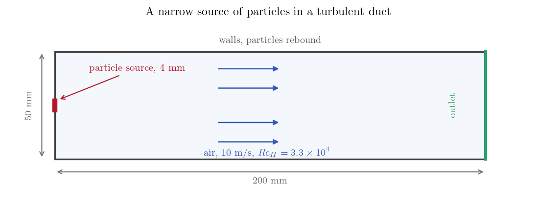
Figure 1: The duct. Particles enter through a 4 mm patch at mid-height, the air through the whole inlet section.

The inlet is split into two zones with the same fluid condition, one of which also carries the particle release. Splitting a boundary by a geometric criterion is the simplest way to obtain a source narrower than the inlet:

<boundary label="source" nature="inlet">X0 and box[-1, 0.023, -1, 0.001, 0.027, 1]</boundary>
<boundary label="inlet"  nature="inlet">X0 and not box[-1, 0.023, -1, 0.001, 0.027, 1]</boundary>

Boundary	Fluid	Particles
source (4 mm of the inlet)	inlet, \(10\) m/s	release of the three classes
rest of the inlet	inlet, \(10\) m/s	rebound
outlet	free outlet	particles leave
walls	no-slip walls	rebound
spanwise planes	symmetry	particle symmetry

Numerical setup

Setting	Value
Mesh	\(100 \times 100 \times 1\) cells (\(2 \times 0.5\) mm)
Turbulence	\(k\)-\(\varepsilon\)
Time step	\(10^{-4}\) s, constant
Iterations	\(12\,000\) (\(1.2\) s)
Statistics start	iteration \(500\)
Release	\(30\) particles per class at every time step

The particles cross the duct in \(20\) ms, so the averaging window covers some fifty transits. The release is continuous, one batch per time step, and the cells are four times finer across the duct than along it, since the quantity being measured is a width of a few millimetres.

Running the simulation

cd Lag_Dispersion_Plume/CASE
code_saturne run --n 4 --id plume

The run takes about thirteen minutes on four cores, almost all of it spent moving particles rather than solving the flow.

Results

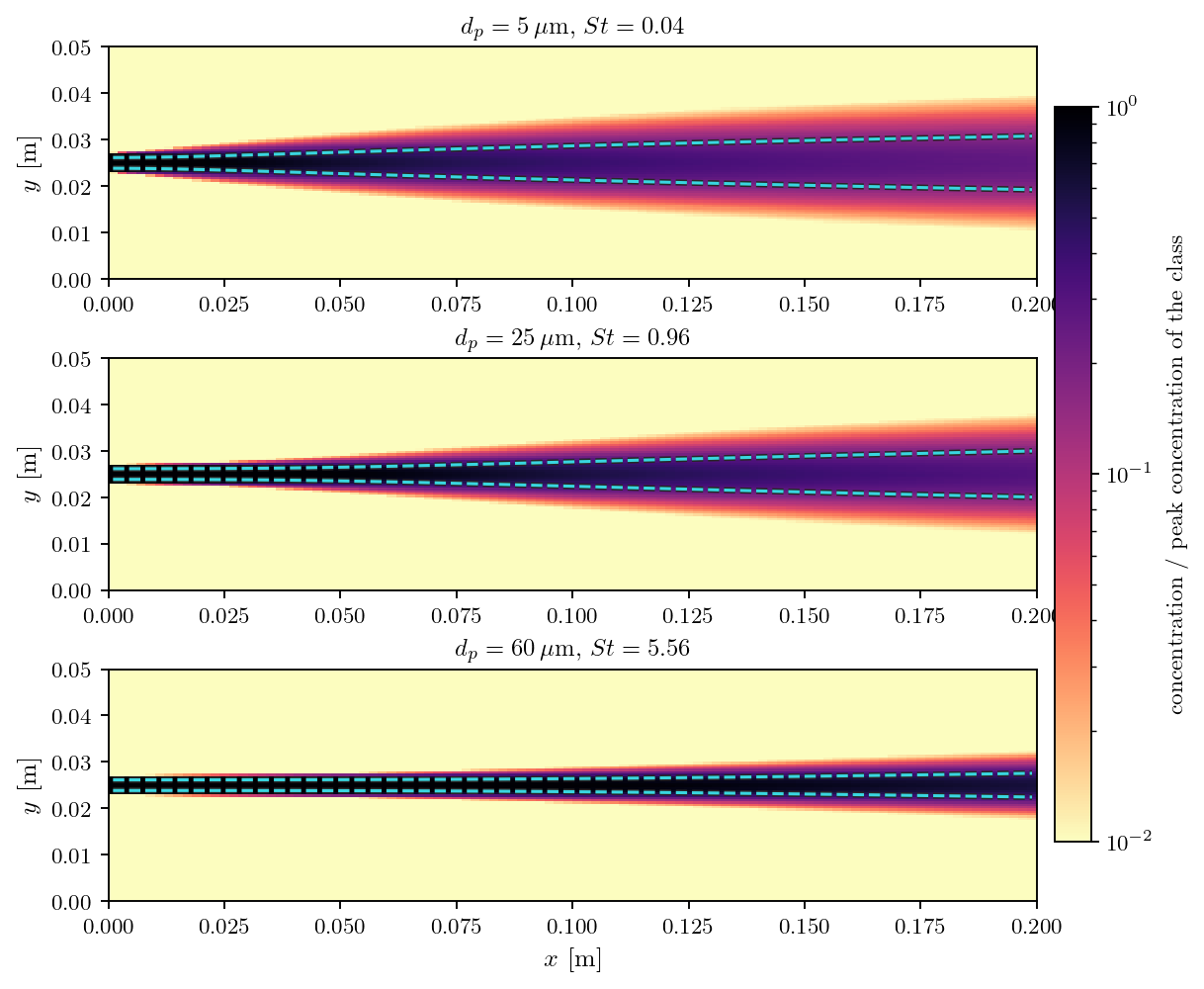
Figure 2: Concentration of each class, from the volume statistics, each panel normalised by its own peak and shown over two decades so the dilute edges of the plume stay visible. The dashed lines mark the plume half width computed from the same field.

All three plumes leave the same 4 mm source with the same fluid velocity, and they spread differently: the 5 micron particles fill a wide band by the end of the duct, the 60 micron ones stay a narrow streak.

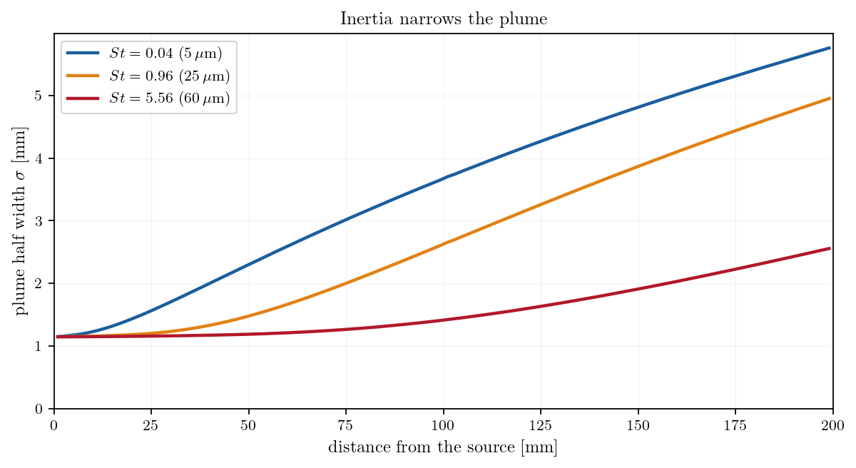
Figure 3: Plume half width along the duct, the standard deviation of the concentration profile at each station.

Measured this way, the heaviest class ends up a little under half as wide as the lightest by the end of the duct. The mechanism is inertia acting as a filter: a particle only responds to eddies that last longer than its relaxation time, so the fast, small-scale motions that spread the light particles pass the heavy ones by. The lightest class, whose relaxation time is short compared with everything in the flow, follows the air closely and disperses almost like a passive scalar would.

Summary

Volume statistics turn a swarm of trajectories into concentration fields, one per particle class, which can then be measured. On a narrow source in a turbulent duct they show inertia filtering the turbulence: the plume of the heaviest particles ends up a little under half as wide as that of the lightest, all else being equal.

Two things to remember. The carrier flow has to be declared steady for these fields to be time averages, and the averaging has to start after the flow has settled.

References

1. code_saturne documentation

Authors

Simvia - Questions, remarks and requests are welcome.