Steady Conjugate Heat Transfer (CHT)

Browse this case on GitHub

This tutorial solves a steady conjugate heat-transfer (CHT) problem with code_saturne. A laminar incompressible flow passes over three hollow solid cylinders aligned with the streamwise direction. Each cylinder is heated from its inner core, heat is conducted through the solid annulus, and the resulting thermal flux is transferred to the surrounding fluid through internally coupled fluid-solid interfaces.

The supplied setup is configured for code_saturne 9.1 and uses a pseudo-steady local time-stepping procedure to converge the coupled flow and temperature solution.

Maintained by Simvia, part of the tutoriel-code_saturne collection.

Learning objectives

After completing this tutorial, the user should be able to:

1. Define separate fluid and solid volume zones in a single code_saturne mesh.
2. Activate the temperature equation and internal fluid-solid coupling for the thermal scalar.
3. Prescribe distinct fluid and solid thermal conductivities, with a fixed temperature on the inner cores.
4. Solve a steady laminar incompressible flow with heat transfer and a temperature-dependent density.
5. Converge the problem with the SIMPLEC pseudo-steady algorithm.
6. Visualize the conjugate temperature field and check its physical consistency.

Prerequisites

Requirement	Detail
code_saturne	v9.1
Background	Basic notions of convective heat transfer and conduction

If code_saturne is not yet installed, build it from the official homepage, pull a ready-to-use Singularity image from the Open Simulation Center, or pull the Simvia Docker image before continuing.

Case files

Th_Conjugate_Heat_Transfer/
├── CASE/
│   └── DATA/
│       └── setup.xml
├── MESH/
│   └── cht_3cylinders_code_saturne_split_farfield.msh
├── FIGURES/
│   ├── cht_mesh_boundary_conditions.png
│   └── cht_conjugate_temperature.png
└── README.md

Physical model

Fluid region

The fluid is modeled as a steady, laminar, incompressible flow with variable density and heat transfer. Turbulence, gravity, radiation, combustion, and compressibility models are disabled.

The steady mass-conservation equation is

\[ \nabla\cdot(\rho\mathbf{u})=0. \]

The momentum equation may be written as

\[ \nabla\cdot(\rho\mathbf{u}\otimes\mathbf{u}) =-\nabla p +\nabla\cdot\left[\mu\left(\nabla\mathbf{u}+\nabla\mathbf{u}^{T}\right)\right]. \]

The temperature field in the fluid is governed by the steady advection-diffusion equation

\[ \nabla\cdot(\rho c_p\mathbf{u}T) =\nabla\cdot(k_f\nabla T), \]

where \(k_f\) is the fluid thermal conductivity.

The fluid density follows the temperature-dependent law used in setup.xml:

\[ \rho(T)=\rho_{\mathrm{ref}}\frac{T_{\mathrm{ref}}}{T}, \]

with

\[ \rho_{\mathrm{ref}}=2.10322\times10^{-4}\ \mathrm{kg\,m^{-3}}, \qquad T_{\mathrm{ref}}=288.15\ \mathrm{K}. \]

This density scaling is part of the case setup and is chosen together with the viscosity, velocity, and cylinder diameter to obtain the target Reynolds number. It should not be interpreted as standard atmospheric air density.

Solid regions

The three cylinders are defined as solid volume zones named solid1, solid2, and solid3. No momentum equation is solved in the solids. In the steady case, heat conduction is governed by

\[ \nabla\cdot(k_s\nabla T)=0, \]

where \(k_s\) is the solid thermal conductivity.

The inner surface of each hollow cylinder is maintained at

\[ T_{\mathrm{core}}=350\ \mathrm{K}. \]

Heat therefore conducts radially through each solid annulus before being transferred to the surrounding fluid.

Internal conjugate coupling

The thermal scalar temperature is activated for internal coupling, and the three solid volume zones are registered as coupled solid zones. code_saturne automatically constructs the internal fluid-solid interfaces from these volume definitions.

At each coupled interface, the solution must satisfy temperature continuity and conservation of normal heat flux:

\[ T_f=T_s, \]

\[ k_f\frac{\partial T_f}{\partial n} =k_s\frac{\partial T_s}{\partial n}. \]

The interface temperature is therefore not prescribed. It is obtained as part of the coupled solution from the balance between conduction in the solid and convection-diffusion in the fluid.

Flow parameters

The inlet and material properties used by the supplied setup.xml are summarized below.

Fluid properties

Parameter	Value	Unit	Source in setup.xml
Inlet velocity magnitude \(U_\infty\)	3.40297	\(\mathrm{m\,s^{-1}}\)	inlet/velocity_pressure/norm
Inlet temperature \(T_\infty\)	288.15	K	inlet thermal dirichlet
Reference density \(\rho_{\mathrm{ref}}\)	\(2.10322\times10^{-4}\)	\(\mathrm{kg\,m^{-3}}\)	density/formula
Dynamic viscosity \(\mu\)	\(1.7893\times10^{-5}\)	\(\mathrm{Pa\,s}\)	molecular_viscosity
Specific heat \(c_p\)	1004.703	\(\mathrm{J\,kg^{-1}\,K^{-1}}\)	specific_heat
Thermal conductivity \(k_f\)	0.024968265	\(\mathrm{W\,m^{-1}\,K^{-1}}\)	thermal_conductivity

Using the outer cylinder diameter \(D=1\ \mathrm{m}\), the inlet Reynolds number is

\[ Re_D=\frac{\rho_{\mathrm{ref}}U_\infty D}{\mu}\approx40. \]

The corresponding Prandtl number is

\[ Pr=\frac{c_p\mu}{k_f}\approx0.72. \]

The low Reynolds number supports the laminar-flow assumption used in this tutorial.

Solid properties

For the steady conduction problem only the solid conductivity and the imposed core temperature enter the solution (density and specific heat play no role at steady state). All three solid zones use the same values:

Parameter	Value	Unit	Source in setup.xml
Thermal conductivity \(k_s\)	0.1028	\(\mathrm{W\,m^{-1}\,K^{-1}}\)	thermal_conductivity solid-zone formula
Inner-core temperature	350	K	core1/2/3 wall dirichlet

The solid conductivity is approximately \(4.12\) times the fluid conductivity:

\[ \frac{k_s}{k_f}\approx4.12. \]

For the present steady problem, the thermal conductivity directly controls the conductive temperature gradient through the solid annuli.

Geometry and boundary conditions

Geometry

Three identical hollow cylinders are arranged in-line along \(x\), centered at \((0.5,0)\), \((5.5,0)\) and \((10.5,0)\ \mathrm{m}\). Each has an outer radius of \(0.5\ \mathrm{m}\) (the fluid-solid interface) and an inner radius of \(0.25\ \mathrm{m}\) (the heated core), so the outer diameter \(D=1\ \mathrm{m}\) is the reference length. They sit inside a circular far-field of radius \(30.5\ \mathrm{m}\) centered at \((5.5,0)\). The domain is extruded by \(1\ \mathrm{m}\) in \(z\) with the front and back planes (\(z=\pm0.5\ \mathrm{m}\)) treated as symmetry, making the calculation quasi-two-dimensional (see Figure 1).

Mesh

The mesh has four volume zones: fluid (33,700 cells) and solid1, solid2, solid3 (4,534 cells each), for a total of 47,302 cells. It is strongly refined around the cylinders and their fluid-solid interfaces, and coarsens toward the far-field boundary.

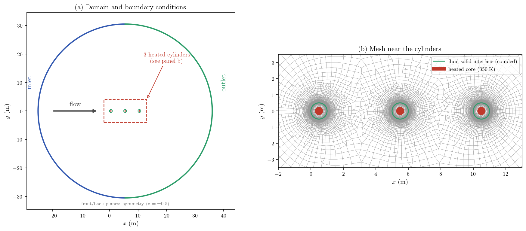
Figure 1: (a) The circular far-field is split into an upstream inlet (blue) and a downstream outlet (green); the three heated cores are at the center. (b) Mesh near the cylinders: the green circles are the internally coupled fluid-solid interfaces and the red disks are the heated cores.

Boundary conditions

Boundary	Type	Thermal condition	Flow condition
inlet	Inlet	\(T=288.15\ \mathrm{K}\)	\(\mathbf{u}=(3.40297,0,0)\ \mathrm{m\,s^{-1}}\)
outlet	Outlet	Zero normal temperature gradient	Standard pressure outlet
core1	Wall	\(T=350\ \mathrm{K}\)	Solid inner boundary
core2	Wall	\(T=350\ \mathrm{K}\)	Solid inner boundary
core3	Wall	\(T=350\ \mathrm{K}\)	Solid inner boundary
front	Symmetry	Symmetry	Symmetry
back	Symmetry	Symmetry	Symmetry
Fluid-solid interfaces	Internal coupling	Temperature and heat-flux continuity	Automatically generated from the solid zones

The outer cylinder surfaces do not require prescribed wall temperatures. Their interface temperatures are determined by the conjugate heat-transfer solution.

Numerical setup

The principal numerical settings in CASE/DATA/setup.xml are:

Setting	Value
Fluid-solid coupling	Internal coupling of temperature
Solid zones	solid1, solid2, solid3
Velocity-pressure algorithm	SIMPLEC
Time treatment	Pseudo-steady local time step
Number of iterations	1500

The pseudo-time used by the steady local-time-step algorithm is a numerical convergence device. Intermediate iteration times should therefore not be interpreted as physical transient time.

Initialization

The fluid is initialized at the inlet conditions (\(\mathbf{u}=(3.40297,0,0)\ \mathrm{m\,s^{-1}}\), \(T=288.15\ \mathrm{K}\)) and the solids at the core temperature (\(T=350\ \mathrm{K}\)).

Running the simulation

The commands below start from the tutorial directory:

cd Th_Conjugate_Heat_Transfer/

Option A: Graphical interface

code_saturne gui CASE/DATA/setup.xml &

The GUI opens the pre-configured setup.xml. Review the setup if you wish, then launch the run with the gear (Run) button in the toolbar. To run in parallel, set the number of processes under Calculation management > Performance settings before launching.

Option B: Command line

The command-line launcher is run from inside the case directory:

cd CASE

# serial
code_saturne run

# parallel (e.g. 4 MPI ranks)
code_saturne run --n 4

Each run creates a time-stamped directory CASE/RESU/<YYYYMMDD-HHMM>/ containing:

• run_solver.log: solver log and residual history,
• monitoring/: probe time series (probes_*.csv),
• postprocessing/: volume and boundary fields in EnSight Gold format.

Results

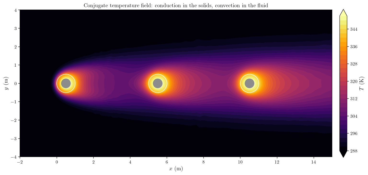
Figure 2: Conjugate temperature field.

Each heated core (350 K) warms its solid annulus; the heat crosses the coupled outer interface and is convected downstream, so a thermal wake trails each cylinder, and the second and third cylinders meet fluid already warmed by the upstream ones. The field is smooth across the fluid-solid interfaces (no artificial jump) and symmetric about the centerline, and the temperature stays between the inlet value (288 K) and the core value (350 K) as expected.

Summary

This tutorial set up a steady conjugate heat-transfer calculation in code_saturne: one laminar fluid region and three solid cylinders in a single mesh, with the temperature equation coupled across the fluid-solid interfaces so the outer cylinder temperatures are part of the solution rather than prescribed. The converged field is bounded, symmetric, and shows the expected conduction in the solids and thermal wakes in the fluid. It is a reproducible internal-CHT set-up rather than a validated benchmark: the flow is quasi-2D and laminar (\(Re_D\approx40\)), gravity and radiation are neglected, the low reference density is a scaling choice (not atmospheric air), and no mesh-independence study or external comparison is included. It is a good starting point for studies of interface heat flux, mesh sensitivity, or higher-Reynolds-number thermal flows.

References

1. code_saturne documentation, Conjugate heat transfer: internal fluid-thermal coupling: https://code-saturne.org/doc/.
2. code_saturne project documentation and user resources: https://www.code-saturne.org/.
3. S. V. Patankar, Numerical Heat Transfer and Fluid Flow, Hemisphere Publishing Corporation, 1980.
4. F. P. Incropera, D. P. DeWitt, T. L. Bergman, and A. S. Lavine, Fundamentals of Heat and Mass Transfer, Wiley.

Authors

Simvia - Questions, remarks and requests are welcome.