Turbulent Heated Channel with Wall Functions (Nusselt vs Gnielinski)
The forced-convection series moves to turbulence: a fully developed turbulent channel flow heated by a uniform wall flux, computed with the high-Reynolds approach of industrial practice, a coarse mesh whose first cell sits in the logarithmic region and wall functions for both the velocity and the temperature. The friction coefficient and the Nusselt number are compared with the Dean and Gnielinski correlations and with a wall-resolved computation on the same case. The channel is streamwise-periodic, driven by a body force that fixes the friction Reynolds number, with the energy sink that keeps the periodic temperature steady.
Maintained by Simvia, part of the tutoriel-code_saturne collection.
Learning objectives
After completing this tutorial you will be able to:
- Set up a wall-function RANS computation with heat transfer: \(k\)-\(\varepsilon\) with the two-scale log law, first cell at \(y^+ \approx 30\), thermal wall function of the temperature scalar.
- Build a streamwise-periodic heated channel: body force in place of the pressure gradient, uniform wall flux, and the user source term that removes the heat input from the periodic temperature.
- Compute \(Cf\), \(y^+\) and \(Nu\) from the solver's boundary fields and check them against the Dean and Gnielinski correlations.
- Know the sensitivity of the result to the wall treatment: \(y^+\) of the first cell, log-law or all-\(y^+\) wall function, wall-resolved reference.
Prerequisites
| Requirement | Detail |
|---|---|
| code_saturne | v9.1 |
| Cases | Inc_Turbulent_Channel (periodic channel, body force), Inc_Streamwise_Periodic (periodic temperature with a source term), Th_Uniform_Flux_Channel |
| Background | Law of the wall, wall functions, turbulent heat transfer correlations |
If code_saturne is not yet installed, build it from the official homepage, pull a ready-to-use Singularity image from the Open Simulation Center, or pull the Simvia Docker image before continuing.
Case files
Th_Turbulent_Heated_Channel/
├── CASE/
│   ├── DATA/
│   │   └── setup.xml                      # mesh, periodicity, body force, turbulence, thermal scalar
│   └── SRC/
│       ├── cs_user_source_terms.cpp       # energy sink of the periodic temperature
│       └── cs_user_extra_operations.cpp   # Cf, y+, Nu and wall-normal profiles
├── FIGURES/
└── README.md
No MESH directory: the mesh is generated at run time by the cartesian mesher. The source-term routine is mandatory (periodic temperature); the other one is a post-processing.
Physical model
Air with constant properties (\(\rho = 1.2\) kg/m³, \(\nu = 1.5 \times 10^{-5}\) m²/s, \(c_p = 1005\) J/kg/K, \(\lambda = 0.0257\) W/m/K, \(Pr = 0.70\)) flows between two parallel walls separated by \(2h = 100\) mm. The flow is fully developed and streamwise-periodic: the velocity field repeats itself, while the pressure drops and the temperature rises linearly along \(x\) (Patankar, Liu and Sparrow, 1977). The two linear drifts become source terms of the periodic problem:
- the momentum receives the body force \(f_x = \rho u_\tau^2/h = 2.16\) N/m³, which fixes the wall shear stress \(\tau_w = f_x h\) and the friction Reynolds number \(Re_\tau = u_\tau h/\nu = 1000\) (\(u_\tau = 0.3\) m/s); the bulk velocity is a result, \(U_b \approx 5.9\) m/s, \(Re_{D_h} = U_b D_h/\nu \approx 8 \times 10^{4}\) with \(D_h = 4h\);
- the energy receives a sink equal to the heat input of the walls, weighted by the local streamwise velocity, so that the periodic temperature \(\tilde{T}\) is statistically steady; the Nusselt number only involves differences of \(\tilde{T}\) and is unaffected by the drift.
Both walls transfer \(q_w = 100\) W/m² to the fluid. The quantities compared with the references are
References. Dean's correlation for plane channels, \(Cf = 0.073\,Re_{2h}^{-1/4}\), and Gnielinski's correlation for the Nusselt number, \(Nu = (f/8)(Re_{D_h} - 1000)Pr / \left(1 + 12.7\sqrt{f/8}\,(Pr^{2/3} - 1)\right)\) with \(f = (0.79\ln Re_{D_h} - 1.64)^{-2}\), both with an uncertainty of about \(\pm 10\%\) (Gnielinski is a pipe correlation applied with \(D_h\)). A wall-resolved \(k\)-\(\omega\) SST run of the same case (\(y^+ = 1\), 150 cells) serves as the internal reference.
Wall functions. With the first cell centre at \(y^+ \approx 30\), the wall shear stress and the wall heat flux are not computed from the resolved gradients but from the logarithmic laws: the two-scale log law of code_saturne for the velocity (friction velocity from the turbulent kinetic energy, \(u_k = C_\mu^{1/4} k^{1/2}\)) and the Arpaci-Larsen thermal law for the temperature, the default for scalars. The log-law wall function requires the first cell in the logarithmic region, \(30 \lesssim y^+ \lesssim 300\).
Geometry and boundary conditions
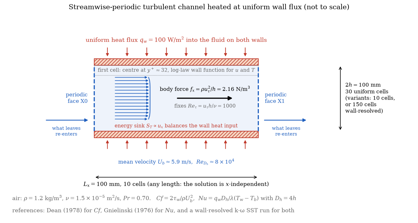
Figure 1: The case. A streamwise-periodic channel driven by a body force, heated by a uniform flux, with the first cell in the logarithmic region.
The domain is \(0.1 \times 0.1 \times 0.01\) m meshed with \(10 \times 30 \times 1\) uniform cells: the first cell centre is at \(1.67\) mm from the wall, \(y^+ = 32\). The streamwise length is arbitrary.
| Boundary | Nature | Condition |
|---|---|---|
X0, X1 |
Translational periodicity | |
walls (Y0, Y1) |
Wall | no slip, temperature prescribed flux \(-100\) W/m² (heating) |
Z0, Z1 |
Symmetry |
The body force is entered in the GUI as a momentum source term on the volume zone (Su = 2.16;). The initial velocity is \(6\) m/s and the initial temperature \(300\) K.
Numerical setup
| Setting | Value |
|---|---|
| Turbulence | \(k\)-\(\varepsilon\) linear production, wall function two-scale log law (option 3 in the GUI) |
| Thermal scalar | temperature, SGDH turbulent flux with the default turbulent Prandtl number \(\sigma_t = 1\), Arpaci-Larsen thermal wall function (default, reported as iwalfs in setup.log) |
| Steady algorithm | local (pseudo) time step, reference \(0.01\) s, SIMPLEC, \(10000\) iterations |
| Energy sink | cs_user_source_terms.cpp, \(S_T = q_w A_w/V \times u_x/\langle u_x \rangle\) |
| Post-processing | cs_user_extra_operations.cpp: \(U_b\), \(T_b\), wall averages of \(T_w\), \(\tau_w\), \(y^+\), \(q_w\), then \(Cf\), \(Re_{D_h}\), \(Nu\) in channel_summary.csv; profiles of one column of cells in profiles.csv |
The run takes about ten seconds in serial.
Variants used in the comparison
Three variants of the shipped case are reported below; each is one or two edits in the GUI:
| Variant | Edit |
|---|---|
| first cell at \(y^+ = 96\) | Mesh > Cartesian mesh: 10 cells in \(y\) instead of 30 |
| \(k\)-\(\omega\) SST with the all-\(y^+\) wall function | Turbulence models: \(k\)-\(\omega\) SST, wall function "All y+ (2-scale model)" |
| wall-resolved \(k\)-\(\omega\) SST (reference) | same model, wall function "No wall function", 150 cells in \(y\) with the parabolic law and ratio \(1.04\) |
Running the simulation
cd Th_Turbulent_Heated_Channel/CASE
code_saturne run
The run writes run_solver.log (the summary line Channel summary: ... at the end), channel_summary.csv, profiles.csv and the EnSight output. The routines are written for a serial run.
Results and verification
| Wall treatment | \(y^+\) | \(Re_{D_h}\) | \(Cf\) | Dean | \(Nu\) | Gnielinski | \(T_w - T_b\) [K] |
|---|---|---|---|---|---|---|---|
| \(k\)-\(\varepsilon\), log-law wall function (shipped case) | \(32\) | \(83100\) | \(0.00464\) | \(0.00511\) (\(-9\%\)) | \(143.9\) | \(155.1\) (\(-7\%\)) | \(5.41\) |
| \(k\)-\(\varepsilon\), log-law wall function, coarser | \(96\) | \(82100\) | \(0.00471\) | \(0.00513\) (\(-8\%\)) | \(145.3\) | \(153.6\) (\(-5\%\)) | \(5.36\) |
| \(k\)-\(\omega\) SST, all-\(y^+\) wall function | \(33\) | \(80000\) | \(0.00497\) | \(0.00516\) (\(-4\%\)) | \(149.2\) | \(150.5\) (\(-1\%\)) | \(5.22\) |
| \(k\)-\(\omega\) SST, wall-resolved (reference) | \(1\) | \(80200\) | \(0.00491\) | \(0.00516\) (\(-5\%\)) | \(155.2\) | \(150.9\) (\(+3\%\)) | \(5.01\) |
- The friction Reynolds number is recovered exactly by every run (\(Re_\tau = 1000\), the body force fixes \(\tau_w\)); what differs between wall treatments is the bulk velocity, hence \(Cf\) and \(Re_{D_h}\).
- The wall-function \(k\)-\(\varepsilon\) gives \(Cf\) and \(Nu\) within \(7\) to \(9\%\) of the correlations, on the low side, and within \(5\%\) of the wall-resolved reference for \(Cf\) and \(7\%\) for \(Nu\): the usual accuracy of the high-Reynolds approach. Moving the first cell from \(y^+ = 32\) to \(96\) changes the results by \(1\) to \(2\%\): the method is insensitive to the mesh as long as the first cell stays in the logarithmic region, which is its purpose.
- The all-\(y^+\) wall function with \(k\)-\(\omega\) SST on the same coarse mesh is within \(1\%\) of Gnielinski and \(4\%\) of Dean.
- The wall-resolved reference itself sits \(5\%\) below Dean and \(3\%\) above Gnielinski: the correlations carry their own uncertainty, and the spread between all four results, about \(8\%\) on \(Nu\), is the realistic accuracy of RANS heat transfer on this configuration.
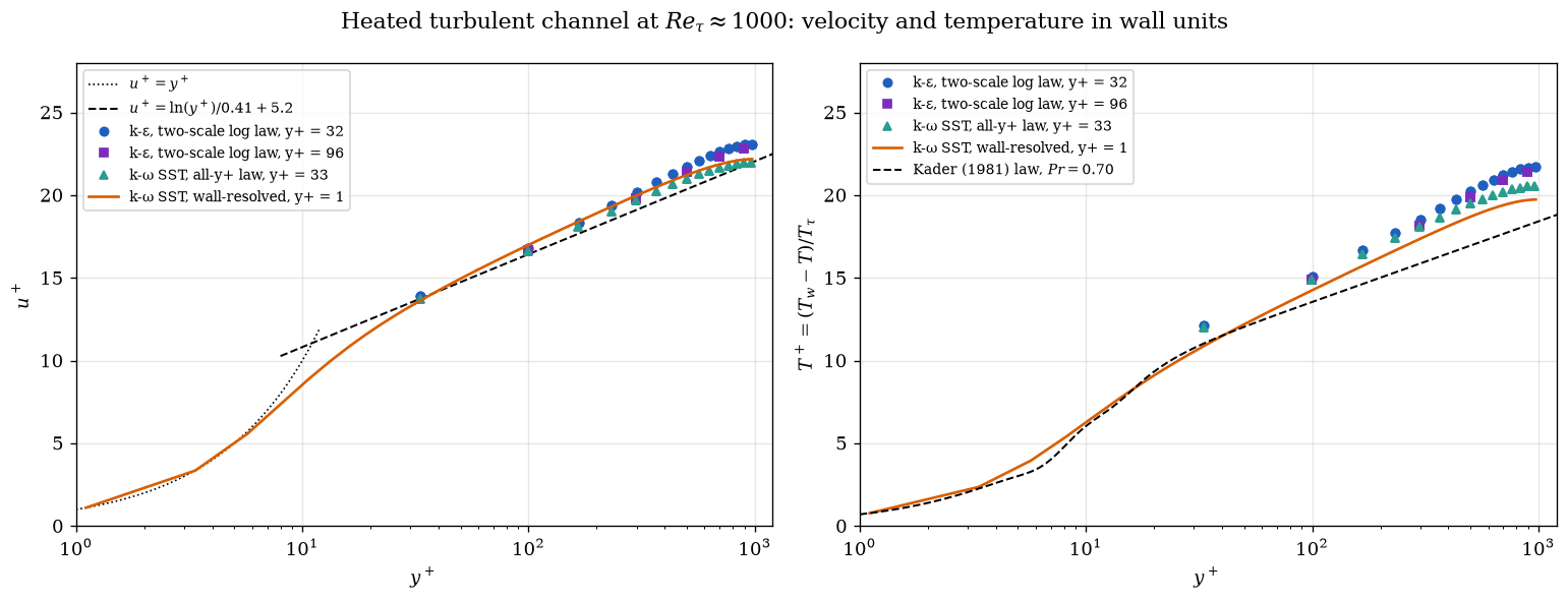
Figure 2: Mean velocity (left) and temperature (right) in wall units for the four wall treatments, against the logarithmic law of the wall and the thermal law of Kader (1981).
The wall-function runs have no point below \(y^+ = 30\): their first cell sits on the logarithmic law by construction, and the profiles above it follow the law of the wall and the wall-resolved profile. The temperature profiles depart from Kader's law in the outer region (\(y^+ > 100\)), where the channel core is not a boundary layer; the four treatments agree there within \(1\) \(T^+\) unit, the \(k\)-\(\varepsilon\) runs being slightly above the SST ones, which is the \(7\%\) difference in \(Nu\).
Summary
A streamwise-periodic turbulent channel heated at uniform flux, computed with \(k\)-\(\varepsilon\) and wall functions on a 300-cell mesh in ten seconds, gives the friction coefficient and the Nusselt number within \(7\) to \(9\%\) of the Dean and Gnielinski correlations and is insensitive to the first-cell \(y^+\) between \(30\) and \(100\). The all-\(y^+\) wall function of \(k\)-\(\omega\) SST does better on the same mesh, and a wall-resolved run brackets the correlations from the other side: the tutorial gives the order of magnitude of the accuracy to expect from RANS wall treatments on heat transfer, and the workflow to check it.
References
- S.V. Patankar, C.H. Liu, E.M. Sparrow. Fully developed flow and heat transfer in ducts having streamwise-periodic variations of cross-sectional area, Journal of Heat Transfer, 99:180-186, 1977.
- V. Gnielinski. New equations for heat and mass transfer in turbulent pipe and channel flow, International Chemical Engineering, 16:359-368, 1976.
- R.B. Dean. Reynolds number dependence of skin friction and other bulk flow variables in two-dimensional rectangular duct flow, Journal of Fluids Engineering, 100:215-223, 1978.
- B.A. Kader. Temperature and concentration profiles in fully turbulent boundary layers, International Journal of Heat and Mass Transfer, 24:1541-1544, 1981.
- code_saturne documentation
Authors
Simvia - Questions, remarks and requests are welcome.