Water Hammer in a Closed Pipe (Stiffened Gas)¶

Browse this case on GitHub

A tutorial on the stiffened gas equation of state of the compressible module of code_saturne, which makes it a solver for pressure waves in liquids: a column of water moving at 1 m/s in a closed pipe is stopped by the end walls, and the pressure surge travels back and forth between them. The pressure history at the wall is validated against the Joukowsky formula $\Delta p = \rho c u_0$ and the period $2L/c$ of the linear acoustic solution.

Maintained by Simvia, part of the tutoriel-code_saturne collection.

Learning objectives¶

After completing this tutorial you will be able to:

Select the stiffened gas law of the compressible module and fit its constants to a liquid (density and sound speed at a reference state).
Set the specific heats the law needs, which the GUI cannot provide for this equation of state.
Initialize a compressible case fully from the GUI with notebook variables (pressure, temperature, velocity).
Validate a water hammer against the Joukowsky formula and the acoustic period, and read the numerical diffusion of the fronts after several reflections.

Prerequisites¶

Requirement	Detail
code_saturne	v9.1
Case	Comp_Sod_Tube (compressible module, cartesian mesh, fixed time step)
Background	Linear acoustics, method of characteristics

If code_saturne is not yet installed, build it from the official homepage, pull a ready-to-use Singularity image from the Open Simulation Center, or pull the Simvia Docker image before continuing.

Case files¶

Comp_Water_Hammer/
├── CASE/
│   ├── DATA/
│   │   └── setup.xml                      # mesh, walls, initial state, notebook, probes, 1D profile
│   └── SRC/
│       └── cs_user_parameters.cpp         # stiffened gas law and its constants
├── FIGURES/
└── README.md

No MESH directory: the mesh is generated at run time by the cartesian mesher. The single user routine selects the equation of state, which the GUI does not offer; everything else is defined in setup.xml.

Physical model¶

The water obeys the Euler equations with the stiffened gas law

\[ p = (\gamma - 1)\,\rho\, e - \gamma\, \Pi, \qquad T = \frac{e - \Pi/\rho}{c_v}, \qquad c = \sqrt{\frac{\gamma\,(p + \Pi)}{\rho}}, \]

an ideal gas shifted by the pressure $\Pi$, which makes the fluid nearly incompressible: with $\Pi \gg p$ the sound speed hardly depends on the pressure. The three constants are fitted so that water at $p_0 = 1$ bar and $T_0 = 300$ K has $\rho_0 = 1000$ kg/m³ and $c = 1500$ m/s with $c_v = 4180$ J/kg/K:

Constant	Relation	Value
$\gamma$	$\gamma(\gamma - 1) = c^2/(c_v T_0)$	$1.9311$
$\Pi$	$\rho_0 (\gamma - 1) c_v T_0 - p_0$	$1.16753 \times 10^{9}$ Pa
$c_p$	$\gamma c_v$	$8072$ J/kg/K

The resulting sound speed is $c = 1501.6$ m/s. These constants reproduce the density and the compressibility of water at the reference state only; they are not meant for large temperature excursions.

The water hammer¶

A pipe of length $L = 1$ m closed at both ends contains water at $p_0$ and $T_0$ moving at $u_0 = 1$ m/s. Unlike the textbook water hammer, where a valve closes at the end of a pipe fed by a reservoir and a single wave is created, both ends act at once: at $t = 0$ the fluid is stopped by the right wall and pulled away from the left wall. A compression wave $+\rho c u_0$ leaves the right wall along the $C^-$ characteristic and a rarefaction $-\rho c u_0$ leaves the left wall along $C^+$, both at speed $c$. They cross at mid-tube at $t = L/(2c)$, where the pressure jumps cancel and the velocity reverses to $-u_0$; each wave then reflects on the opposite wall with the opposite sign, and the whole pattern repeats with the period $2L/c$ (it would be $4L/c$ with a reservoir at one end).

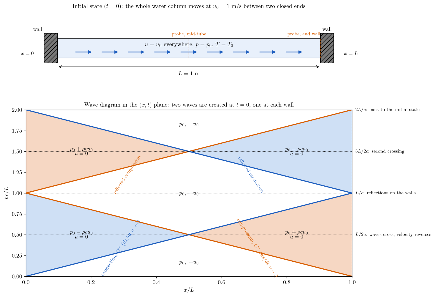
Sketch of the closed pipe with the initial velocity and the two probes, and the wave diagram in the x-t plane with the compression and rarefaction characteristics, their crossing and their reflections.
Figure 1: The initial state (top) and the wave diagram in the $(x, t)$ plane (bottom): the compression created at the right wall and the rarefaction created at the left wall cross at mid-tube, reflect, and restore the initial state after $2L/c$. Shaded regions are at rest, white regions move at $\pm u_0$.

For $u_0 \ll c$ the linear acoustic solution is exact: at the right wall the pressure is a square wave of amplitude $\pm \rho c u_0 = \pm 15.0$ bar and period $2L/c = 1.332$ ms; at mid-tube the pressure stays at $p_0$ and the velocity alternates between $+u_0$ and $-u_0$ every $L/c$. The density follows the pressure with $\Delta \rho = \Delta p / c^2 = 0.67$ kg/m³: a change of $0.07\%$ only, which is the whole compressibility the wave relies on.

Geometry and boundary conditions¶

Thin box of $1 \times 0.01 \times 1$ m meshed with $1000 \times 1 \times 1$ cells ($\Delta x = 1$ mm). The two ends are walls, the four lateral faces symmetry planes. The initial state is set from the GUI on the whole domain with the notebook variables p0, t0 and u0 (pressure, temperature and velocity formulas): pressure and temperature are the two imposed thermodynamic variables, the density and energy follow from the stiffened gas law.

Boundary	Nature	Zone / selection
`x0`, `x1`	Wall	`X0`, `X1`
`y0`, `y1`, `z0`, `z1`	Symmetry	`Y0`, `Y1`, `Z0`, `Z1`

With the default pressure treatment of the compressible module at walls (icfgrp = 1, homogeneous Neumann), symmetry planes at the ends give exactly the same result.

Numerical setup¶

Setting	Value
Equation of state	`ieos = CS_EOS_STIFFENED_GAS`, `gammasg`, `psginf`, `cv0`, `cp0` set in `cs_user_parameters.cpp`
Convection schemes	1st-order upwind (imposed by the compressible module)
Time step	fixed, $4 \times 10^{-7}$ s, $13735$ iterations, $t_{end} = 5.494$ ms $= 8.25\,L/c$, CFL $= 0.6$
Viscosity, conductivity	water values, $10^{-3}$ Pa.s and $0.6$ W/m/K, constant
Probes	$x = 0.9995$ m (end wall) and $x = 0.5005$ m, every time step
1D output	`profiles` block, CSV at the end

Two settings the GUI cannot make. For the stiffened gas, $c_v$ is not deduced from $c_p$ and the molar mass as for an ideal gas: cv0 must be set in cs_user_parameters.cpp, together with cp0 = gamma * cv0. And the viscosity must not be zero: the zero user laws used by the inviscid tutorials make the wall $y^+$ undefined, and the NaN check of the solver stops the run. The real viscosity of water has no visible effect on the waves.

Running the simulation¶

cd Comp_Water_Hammer/CASE
code_saturne run

The run takes about $30$ s in serial and writes run_solver.log, monitoring/probes_<variable>.csv (time histories at the two probes), profiles/tube.csv (profile at $t_{end}$) and the EnSight output. The initial velocity can be changed from the command line, for instance code_saturne run --notebook-args u0=2.

Results and verification¶

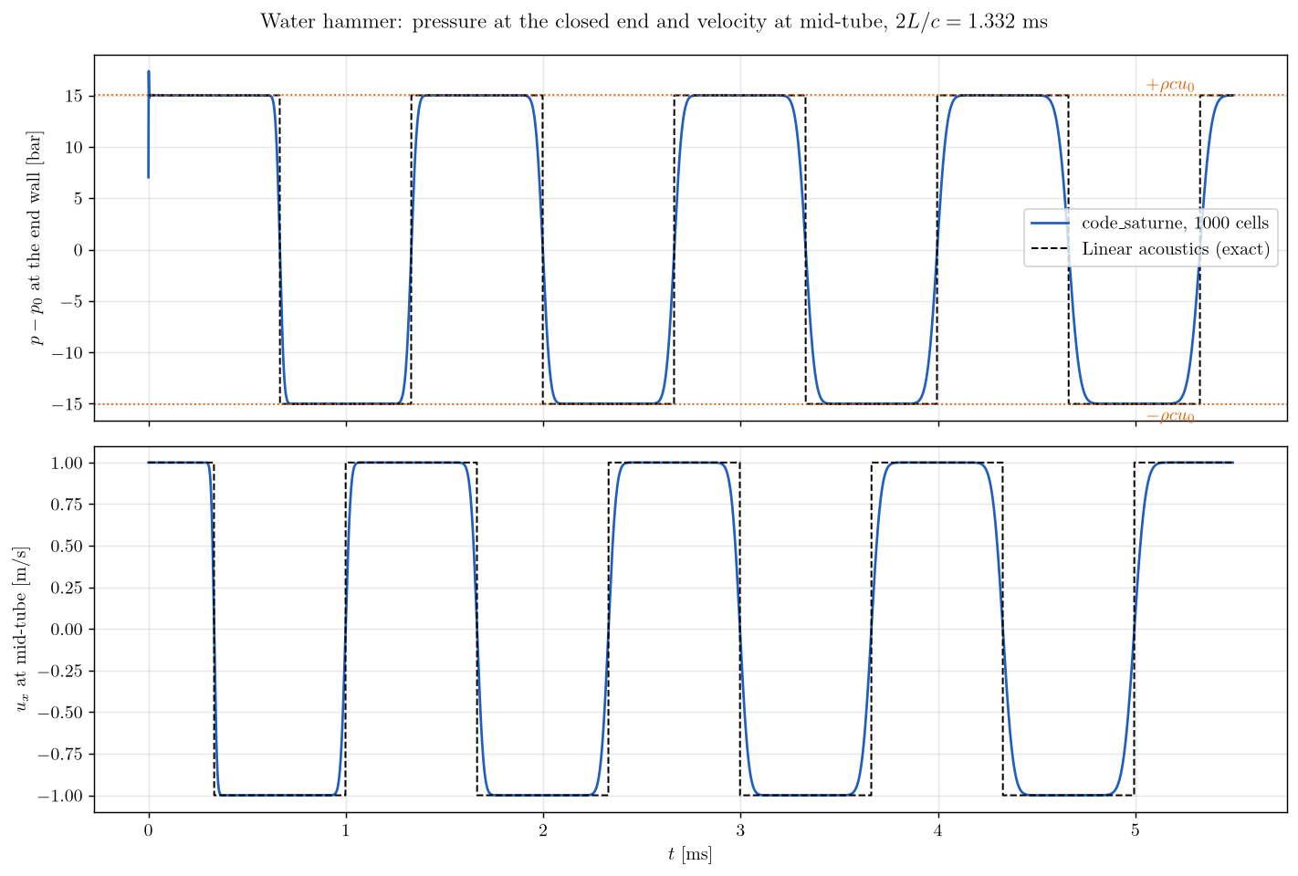
Pressure at the closed end and velocity at mid-tube versus time: code_saturne against the exact square waves of linear acoustics, with the Joukowsky levels.
Figure 2: Pressure at the end wall (top) and velocity at mid-tube (bottom), code_saturne (solid) against the linear acoustic solution (dashed). The dotted lines are the Joukowsky levels $\pm \rho c u_0$.

The first pressure plateau at the wall is $15.02$ bar above $p_0$, the Joukowsky value $\rho c u_0 = 15.016$ bar to $0.05\%$. After seven reflections the plateau is still within $0.5\%$ of it. The density at the wall oscillates between $999.36$ and $1000.80$ kg/m³, as $\Delta p / c^2$ predicts.
The velocity at mid-tube reverses at $t = 0.3336$ ms (exact $L/(2c) = 0.3330$ ms): the wave speed is recovered to $0.3\%$. The sign changes of the wall pressure are spaced by $0.666$ ms, exactly $L/c$.
The fronts widen with each reflection: the 10-90% fall time at the wall grows from $42$ µs after the first reflection to $113$ µs after the seventh, the numerical diffusion of the first-order scheme on a discontinuity that is never steepened.

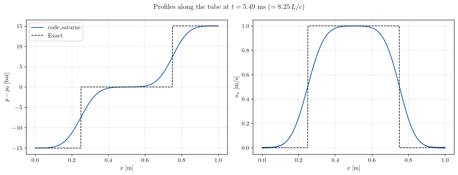
Figure 3: Pressure and velocity along the tube at $t_{end} = 8.25\,L/c$, code_saturne (solid) against the exact solution (dashed).

At $t_{end}$ the two fronts sit at $x = 0.25$ and $0.75$ m: the plateaus ($-15$, $0$ and $+15$ bar; $0$, $u_0$ and $0$) are exact, and each front, which has been reflected eight times, is spread over about $0.18$ m (10 to 90 %). The temperature varies by $\pm 0.19$ K only: the compression of a liquid is almost isothermal, as the stiffened gas law with a large $\Pi$ implies.

Summary¶

With the stiffened gas law and three constants fitted to the density and the sound speed of water, the compressible module computes a water hammer whose surge amplitude and period match the Joukowsky formula and the acoustic solution to a fraction of a percent. The case needs one user routine, because the GUI does not expose this equation of state nor the specific heats it requires, and a non-zero viscosity at the walls. The first-order upwind scheme preserves the plateaus but smears the fronts a little more at each reflection.

References¶

M.H. Chaudhry. Applied Hydraulic Transients, 3rd edition, Springer, 2014 (chapter 2, Joukowsky formula and the water hammer diagram).
E.F. Toro. Riemann Solvers and Numerical Methods for Fluid Dynamics, 3rd edition, Springer, 2009 (chapter 1, stiffened gas law).
code_saturne documentation

Authors¶

Simvia - Questions, remarks and requests are welcome.

Constant	Relation	Value
\(\gamma\)	\(\gamma(\gamma - 1) = c^2/(c_v T_0)\)	\(1.9311\)
\(\Pi\)	\(\rho_0 (\gamma - 1) c_v T_0 - p_0\)	\(1.16753 \times 10^{9}\) Pa
\(c_p\)	\(\gamma c_v\)	\(8072\) J/kg/K