Two-Phase Shock Tube (Compressible Homogeneous Model)
A tutorial on the compressible homogeneous two-phase model of code_saturne: a steam-water mixture with one velocity, one pressure and three transported steam fractions, each phase following a stiffened gas law. The case is the two-phase Riemann problem of Helluy, Hurisse and Le Coupanec (2016), whose exact solution has three constant states. A second run switches on the return to thermodynamic equilibrium and checks that the mixture locks onto the saturation curve.
This model is distinct from the incompressible VOF "homogeneous model" of the GUI (series 50_vof).
Maintained by Simvia, part of the tutoriel-code_saturne collection.
Learning objectives
After completing this tutorial you will be able to:
- Activate the two-phase variant of the compressible module and define a stiffened gas per phase from
cs_user_parameters.cpp(the model has no GUI panel). - Initialize a two-phase state from density, total energy and the three fractions.
- Validate a frozen two-phase mixture against the exact solution of a Riemann problem.
- Apply the return-to-equilibrium step from a user routine and verify \(T = T_{sat}(p)\).
Prerequisites
| Requirement | Detail |
|---|---|
| code_saturne | v9.1 |
| Case | Comp_Sod_Tube (compressible module, cartesian mesh, fixed time step) |
| Background | Gas dynamics; saturation and chemical potential of a two-phase mixture |
If code_saturne is not yet installed, build it from the official homepage, pull a ready-to-use Singularity image from the Open Simulation Center, or pull the Simvia Docker image before continuing.
Case files
Comp_Two_Phase_Shock_Tube/
├── CASE/
│   ├── DATA/
│   │   └── setup.xml                      # mesh, time stepping, notebook, 1D profile output
│   └── SRC/
│       ├── cs_user_parameters.cpp         # model activation, EOS, stiffened gas parameters
│       ├── cs_user_initialization.cpp     # left and right states of the Riemann problem
│       └── cs_user_extra_operations.cpp   # return-to-equilibrium step (notebook switch)
├── FIGURES/
└── README.md
No MESH directory: the mesh is generated at run time by the cartesian mesher. The three user routines are mandatory: the model cannot be set up from the GUI.
Physical model
The mixture has a single velocity \(u\), density \(\rho\) and total energy \(E\), and obeys the Euler equations. Three fractions of the steam, volume \(\alpha\), mass \(y\) and energy \(z\), are transported by the flow and relax towards their equilibrium values with a time scale \(\tau\):
The phasic states follow from the fractions (\(\tau_1 = \alpha \tau / y\), \(e_1 = z e / y\), and similarly for phase 2), and the mixture pressure and temperature combine the phasic laws: \(1/T = z/T_1 + (1-z)/T_2\) and \(p/T = \alpha p_1/T_1 + (1-\alpha) p_2/T_2\). The equilibrium fractions are those for which both phases share the same pressure, temperature and chemical potential at the given \((e, \tau)\). With \(\tau \to \infty\) the mixture is frozen (run 1); with the code default \(\tau = 10^{-30}\) s the return to equilibrium is instantaneous (run 2).
Each phase is a stiffened gas, \(p_k = (\gamma_k - 1)\, e_k/\tau_k - \gamma_k \Pi_k\), \(T_k = (e_k - \Pi_k \tau_k)/c_{v,k}\), with the parameters of the reference, fitted on steam-water properties around 81 bar:
| Phase | Index in the code | \(c_v\) [J/kg/K] | \(\gamma\) | \(\Pi\) [Pa] | \(q'\) [J/kg/K] |
|---|---|---|---|---|---|
| Steam | 0 (fractions transported) | \(4477.8158\) | \(1.0848754\) | \(0\) | \(-49292.11\) |
| Liquid water | 1 | \(1395.2862\) | \(1.6651280\) | \(3.7258761 \times 10^{8}\) | \(0\) |
The entropy constant \(q'\) fixes the saturation curve: the steam value is set so that \(T_{sat}(81\ \mathrm{bar}) = 569\) K as in the reference. The reference energy \(q\) must stay zero in v9.1.
The Riemann problem
| State | \(\alpha\) | \(y\) | \(z\) | \(\rho\) [kg/m³] | \(u\) [m/s] | \(p\) [Pa] |
|---|---|---|---|---|---|---|
| Left (\(x < 0.5\)) | \(0.1380069\) | \(7.843483 \times 10^{-3}\) | \(1.512816 \times 10^{-2}\) | \(728\) | \(5\) | \(7.69 \times 10^{6}\) |
| Intermediate | \(0.1480069\) | \(8.843483 \times 10^{-3}\) | \(1.612816 \times 10^{-2}\) | \(738\) | \(5\) | \(7.69 \times 10^{6}\) |
| Right (\(x \geq 0.5\)) | \(0.1480069\) | \(8.843483 \times 10^{-3}\) | \(1.612816 \times 10^{-2}\) | \(733\) | \(-0.8170134\) | \(4.029078 \times 10^{6}\) |
The fractions are those of the steam. The exact solution is a contact wave at \(u = 5\) m/s and a shock at \(\sigma = 857.774\) m/s; the \(u - c\) wave has zero amplitude. At \(t = 2 \times 10^{-4}\) s the contact is at \(x = 0.501\) m and the shock at \(x = 0.6716\) m.
The reference prints \(u_R = +0.817\) m/s. The Rankine-Hugoniot relations with the quoted shock speed only hold for \(u_R = -0.817\) m/s, which is the value used here.
Geometry and boundary conditions
The domain is a thin box of \(3 \times 0.01 \times 1\) m meshed with \(3000 \times 1 \times 1\) cells, a 1D problem on a 3D mesh, with symmetry planes on all six faces. In v9.1 the two-phase model only supports closed domains (its inlet and outlet conditions abort on an assertion), so the tube is extended to \([-1, 2]\) m: the waves reflected by the ends stay away from the solution at \(t_{end}\).
The states are set cell by cell in cs_user_initialization.cpp: the internal energy is obtained from \((\alpha, y, z, p, \rho)\) with cs_hgn_thermo_ie, and ithvar = 210000 tells the module that density and total energy are the imposed variables. The GUI initialization by pressure and temperature does not go through the two-phase thermodynamics.
Numerical setup
| Setting | Value |
|---|---|
| Model | CS_COMPRESSIBLE = 2, ieos = CS_EOS_HOMOGENEOUS_TWO_PHASE (cs_user_parameters.cpp) |
| Convection schemes | 1st-order upwind (imposed by the compressible module) |
| Time step | fixed, \(2.5 \times 10^{-7}\) s, \(800\) iterations, \(t_{end} = 2 \times 10^{-4}\) s, CFL \(\approx 0.22\) |
| Viscosities, conductivity | \(0\) (user laws) |
| Return to equilibrium | hgn_relax_eq_st = 0, applied from cs_user_extra_operations when the notebook variable relax is \(1\) |
| 1D output | profiles block, CSV at the end, RESU/<id>/profiles/tube.csv |
In v9.1 the solver calls the relaxation step only when the compressible flag equals \(1\), whereas the fractions exist for the value \(2\). The step is therefore applied from
cs_user_extra_operations.cppat the end of each time step, which is exactly the fractional step of the model.
Running the simulation
cd Comp_Two_Phase_Shock_Tube/CASE

# run 1: frozen mixture
code_saturne run --id frozen

# run 2: instantaneous return to equilibrium
code_saturne run --notebook-args relax=1 --id equilibrium
The GUI (code_saturne gui DATA/setup.xml &) shows the mesh, the time stepping, the notebook variable and the profile, but not the model itself. Each run takes about ten seconds in serial and writes run_solver.log, profiles/tube.csv and the EnSight output.
Results and verification
Run 1: frozen mixture against the exact solution
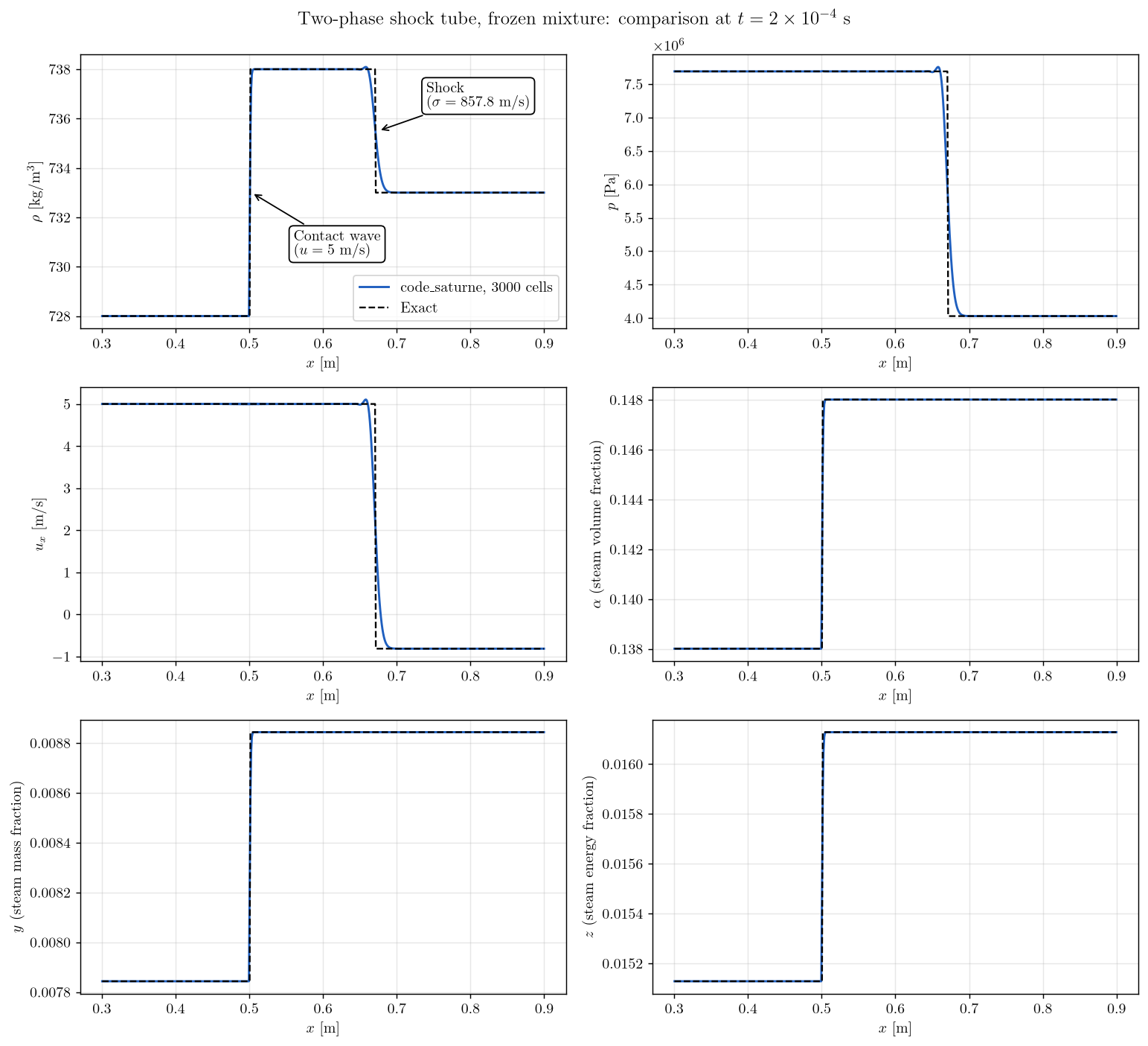
Figure 1: Profiles at $t = 2 \times 10^{-4}$ s, code_saturne (solid) against the exact solution (dashed).
The contact is captured at \(x = 0.5005\) m (exact \(0.501\)) and the shock at \(x = 0.6706\) m (exact \(0.6716\)), the latter spread over about \(0.02\) m with a small overshoot, as in the Sod tube. No wave appears at the \(u - c\) position. \(L^1\) relative errors over \(0 < x < 1\) m:
| \(\alpha\) | \(y\) | \(z\) | \(\rho\) | \(u\) | \(p\) |
|---|---|---|---|---|---|
| \(5.2 \times 10^{-5}\) | \(8.9 \times 10^{-5}\) | \(5.0 \times 10^{-5}\) | \(4.3 \times 10^{-5}\) | \(7.9 \times 10^{-3}\) | \(2.8 \times 10^{-3}\) |
Run 2: instantaneous return to equilibrium
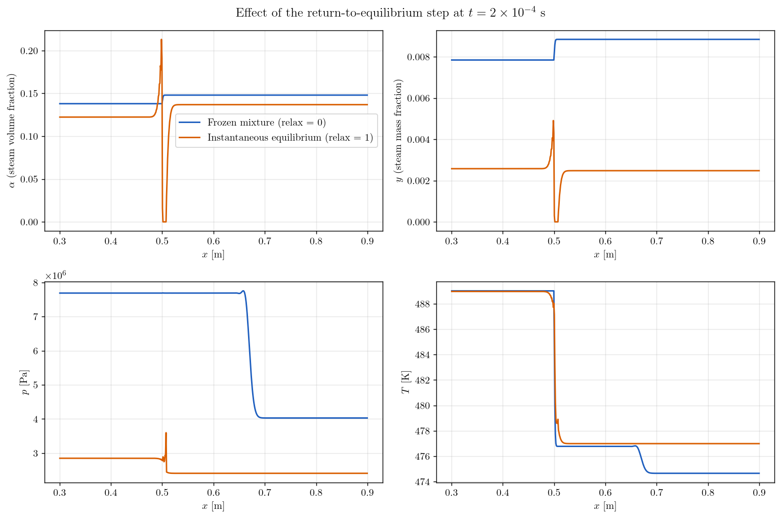
Figure 2: Frozen mixture (blue) against instantaneous return to equilibrium (orange) at $t = 2 \times 10^{-4}$ s.
The initial states are subcooled for the thermodynamics of the model (\(T_{sat}(7.69\ \mathrm{MPa}) = 565\) K against \(489\) K), so the steam condenses from the first time step on:
| Zone | \(p\) [MPa] | \(T\) [K] | \(T_{sat}(p)\) [K] | \(y\) |
|---|---|---|---|---|
| Left plateau, frozen | \(7.69\) | \(489.0\) | \(564.8\) | \(7.84 \times 10^{-3}\) |
| Left plateau, equilibrium | \(2.849\) | \(488.97\) | \(488.97\) | \(2.58 \times 10^{-3}\) |
| Right plateau, frozen | \(4.03\) | \(474.7\) | \(514.5\) | \(8.84 \times 10^{-3}\) |
| Right plateau, equilibrium | \(2.408\) | \(476.99\) | \(476.99\) | \(2.48 \times 10^{-3}\) |
- On every two-phase cell \(|T - T_{sat}(p)| < 10^{-3}\) K: the relaxation brings the mixture onto the saturation curve. The liquid dominates the heat capacity, so the temperature barely moves and the equilibrium is reached by dropping the pressure to \(P_{sat}(T)\).
- The waves have only travelled about \(1.3\) cm instead of \(17\) cm: the effective sound speed of the equilibrium mixture is far below the frozen value, a classical property of homogeneous equilibrium models.
- At the initial discontinuity a pocket of seven cells ends up as pure liquid: on strongly mixed cells the equilibrium search finds no two-phase root and falls back to a single phase. This is a limitation of the algorithm, not a physical feature.
- Mass is conserved exactly and total energy to \(10^{-6}\) in both runs.
Summary
The compressible homogeneous two-phase model is set up entirely from user routines. Without mass transfer the computed Riemann problem matches the exact three-state solution; with the return-to-equilibrium step applied from a user routine, the mixture locks onto the saturation curve of the model. In v9.1 the model is restricted to closed domains, has no GUI support, needs thermodynamic parameters compatible with a hard-coded critical pressure (\(1.5665 \times 10^{8}\) Pa, where a saturation point must exist), and its relaxation step must be called by the user.
References
- P. Helluy, O. Hurisse, E. Le Coupanec. Verification of a two-phase flow code based on an homogeneous model, International Journal on Finite Volumes, 13, 2016.
- O. Hurisse. Application of an homogeneous model to simulate the heating of two-phase flows, International Journal on Finite Volumes, 11, 2014.
- code_saturne documentation
Authors
Simvia - Questions, remarks and requests are welcome.